The Effects of Race, Age, and Income on Home Values: Using Spatial Analysis to Evaluate Ramsey County Homes

Data Context and Research Question

Ramsey County is the most densely populated county in Minnesota. Historically, Minnesota has been welcoming to immigrants, but when the anti-blackness movement was rampant in the US, African-American residents of the Twin Cities were also subject to this discrimination.

During the first few decades of the twentieth century, members of real estate groups in Hennepin and Ramsey County implemented covenants into many housing deeds. These covenants were just a few lines of text in a housing deed that said only people of the “Caucasian race” could rent, lease, or sell various properties throughout the counties (University of Minnesota, n.d.). This went on for many years until the Supreme Court made covenants unenforceable in the late 1940s. However, many real estate companies and property holders ignored this ruling. It was not until 1953 that the Minnesota legislature prohibited them and Congress banned all racial restrictions on housing in 1968 as a part of the Fair Housing Act.

Additionally, the practice of redlining, which involves in marking black neighborhoods as unsafe, effectively bars people of color from receiving quality infrastructure, education, and further restricts them from moving up the social ladder. Moreover, the construction of the Interstate-94 results in the entire Rondo neighborhood, which mostly consists of black residents, being tore down to make way for the highway, causing many to be displaced (Volante 2015.) Despite the fact that these practices happened decades ago, they still had, and are having everlasting impact. Today, while Saint Paul welcomes immigrants from Somalia, Laos, Vietnam, and many other countries and cultures, the city remains highly divided in terms of quality of life, which was carried from the historical legacy.

So, we want to know how these discriminatory policies affect today’s real estate market in Ramsey County. For this research project, we are going to examine the effects of these practices on today’s home values in Ramsey County and see if demographic factors such as race, age, and job sectors can be indicators of Ramsey County’s home values.

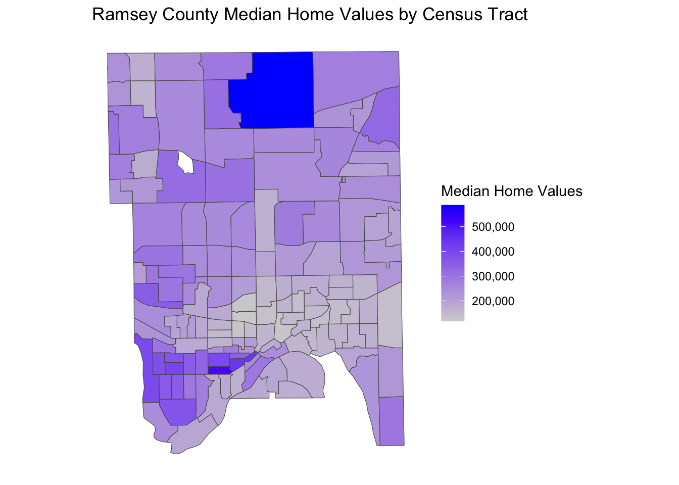
The following visualization shows us how median home values differ between census tracts in Ramsey County. We can see that North Oaks and some neighborhoods in downtown St. Paul (southwest side of the map) have the highest median home values, whereas tracts in central St. Paul tend to have the lowest median home values.

Neighborhood Structure

We chose a rook neighborhood structure as it connects each census tract’s neighbors based on their edges. Doing this will eliminate potential spatial correlation that appears in downtown Saint Paul. If we were to use any distance-based neighborhood structure, there is more likely to be spatial correlation as the census tracts are very condensed in the downtown area. While rook and queen neighborhood structures are similar, we chose not to use a queen as we did not want two tracts to be neighbors if only one point along the borders is touching.

Mean Models

Wb <- nb2listw(Rook, style = "W")
spdep::moran.test(ramsey_data$gam_resid, Wb, alternative = "two.sided", randomisation = TRUE) 

# Find outliers
ramsey_data %>%
    filter(abs(scale(gam_resid)) > 3)

We created two mean models, one utilizing linear regression and the other using splines. We originally chose a linear regression model for median home value as there is a positive linear relationship between median home value and median household income. However, the relationship is not globally linear, so to account for the nonlinearity, we implemented basis splines for BirthPlace_Foreign born:, AgeE, and Industry_Finan.

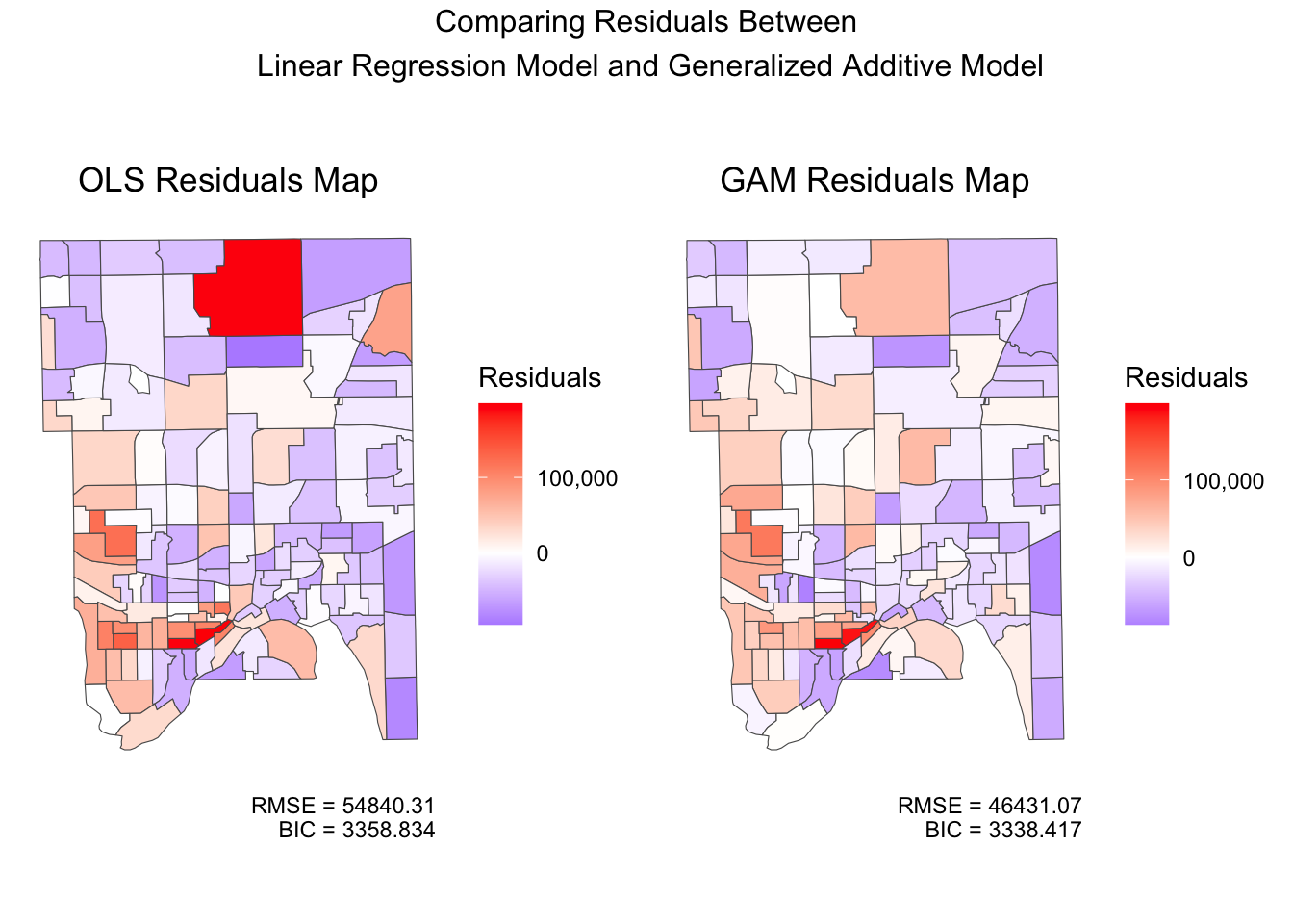
Our visualization shows us that the generalized additive model has a lower BIC score of 3338 and a lower RMSE value of 46431. The linear model does not produce as desirable results as it has a BIC score of 3358 and an RMSE value of 54840.31. Additionally, the generalized additive model better predicts median home values for some census tracts, especially North Oaks. However, the model still overestimates the median home values of census tracts 357 and 358 (downtown St. Paul). After running a Moran’s I test, we found that our model has a p-value of 1.25e-06, so we reject our null hypothesis that there is no spatial correlation. This tells us that we still have some spatial correlation present negatively affecting our model, and we must fit a new model to account for this.

Fitting Spatial Autoregressive Models

# Fit SAR Model
mod_sar <- spautolm(formula = HouseValueE ~ IncomeE +
               bs(`BirthPlace_Foreign born:`, knots = 0.25, degree = 1) + 
               bs(AgeE, knots = 37) + 
               bs(Industry_Finan, knots = 0.06, degree = 1), 
               data = ramsey_data, listw = Wb, family = "SAR")

ramsey_data$sar_resid <- resid(mod_sar)

# Fit CAR Model
mod_car <- spautolm(formula = HouseValueE ~ IncomeE +
               bs(`BirthPlace_Foreign born:`, knots = 0.25, degree = 1) + 
               bs(AgeE, knots = 37) + 
               bs(Industry_Finan, knots = 0.06, degree = 1), 
               data = ramsey_data, listw = Wb, family = "CAR")

ramsey_data$car_resid <- resid(mod_car)

# SAR Eval Metrics
#BIC(mod_sar)
#sqrt(mean(ramsey_data$sar_resid^2))

# CAR Eval Metrics
#BIC(mod_car)
#sqrt(mean(ramsey_data$car_resid^2))

# SAR Moran's I Test
spdep::moran.test(ramsey_data$sar_resid, Wb, alternative = "two.sided", randomisation = TRUE)  # Using randomization test

## 
## 	Moran I test under randomisation
## 
## data:  ramsey_data$sar_resid  
## weights: Wb    
## 
## Moran I statistic standard deviate = 0.13356, p-value = 0.8937
## alternative hypothesis: two.sided
## sample estimates:
## Moran I statistic       Expectation          Variance 
##      -0.000168582      -0.007462687       0.002982444

# CAR Moran's I Test
spdep::moran.test(ramsey_data$car_resid, Wb, alternative = "two.sided", randomisation = TRUE)  # Using randomization test

## 
## 	Moran I test under randomisation
## 
## data:  ramsey_data$car_resid  
## weights: Wb    
## 
## Moran I statistic standard deviate = -0.69209, p-value = 0.4889
## alternative hypothesis: two.sided
## sample estimates:
## Moran I statistic       Expectation          Variance 
##      -0.045448753      -0.007462687       0.003012454

After comparing the outputs of SAR and CAR models, we decided to use SAR. The SAR model not only has lower BIC and RMSE values, but it also has a higher p-value in the Moran’s I test, meaning that we are more confident that the leftover residuals are independent noise/errors. In other words, the SAR model does a better job than the CAR model eliminating the lingering spatial correlation left over from the GAM.

Final Model

Residuals Map

Apparently, GAM fitted SAR reduced the RMSE in a great magnitude. We could also tell the slight changes on the residual map, where the color of SAR residual map is less tinted compared with GAM residual map. It’s a positive signal that the SAR model helped GAM to account more deviations which could caused by the spatial correlation. In other words, the SAR model considered the neighborhood information that could cause the difference/similarity of the house value within a neighborhood.

Coefficient Interpretations

In our model, we assumed IncomeE to have simple linear relationship with HouseValueE, so it only had one slope coefficient which is 2.0810, meaning for each one dollar increase in the census tract’s median income, the estimated median home value will increase by 2.0810 dollars.

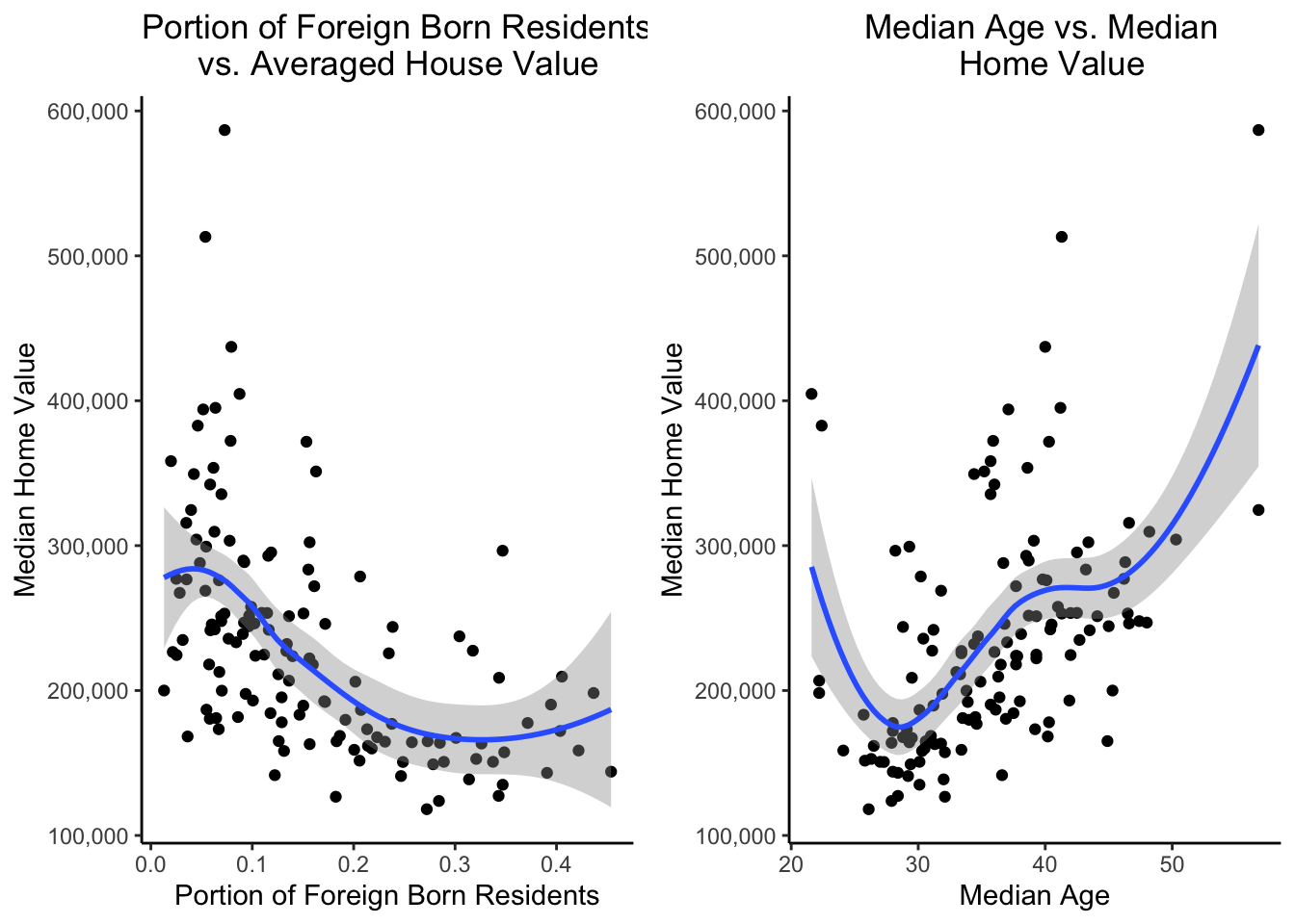
For the variable BirthPlace_Foreign born:, Industry_Finan, and AgeE we used basis spline, so the estimate outputs were hard to interpret, but we could tell a general trend for each variable, especially where its slope changed. For BirthPlace_Foreign born:, we have the knot at 0.25, meaning we expect a drastic change for the slope before and after that knot. From the graph of BirthPlace_Foreign born: vs. HouseValueE, the HouseValueE decreased as the portion of foreign born residents increased, and the decrease of HouseValueE slowed down after the portion of foreign born residents reached 0.25. The relationship between HouseValueE and Industry_Finan shared similar characteristics with HouseValueE vs. BirthPlace_Foreign born:.

For AgeE vs. HouseValueE, the trend of the data has a cubic characteristic, which also being considered within our model of basis spline. From AgeE=27 to AgeE = 37, there’s an increasing trend of HouseValueE. The trend became flat in the range of AgeE=37 to AgeE = 45. And the HouseValueE returned increasing after AgeE=45.

Conclusion

##         RMSE      BIC
## OLS 54840.31 3358.834
## GAM 46431.07 3338.417
## SAR 37401.60 3305.445
## CAR 41705.69 3331.848

Many of the Ramsey County census tracts in downtown St. Paul are highly condensed. We wanted to make sure that even if two census tracts are not direct neighbors, there is still some spatial correlation between the two tracts if they share one or more of the same neighbors. CAR models utilize a spatial modification to the first-order Markov property, meaning that a census tract is only directly influenced by its neighbors (Goodchild and Haining 2004.) SAR models do not follow this property, which is why a SAR model makes more sense in the context of our data. Additionally, our SAR model produces both the lowest RMSE value and BIC score, making it the best model.

References

Goodchild, Michael F, and Robert P Haining. 2004. “GIS and Spatial Data Analysis: Converging Perspectives.” Papers in Regional Science 83 (1): 363–85.

University of Minnesota, Regents of the. n.d. “What Are Covenants?” https://mappingprejudice.umn.edu/what-are-covenants/index.html.

Volante, Alisha J. 2015. “The Rondo Neighborhood & African American History in St. Paul, MN: 1900s to Current.”