Analyzing Boston Home Values
April 25, 2022
Data Context
I chose to use Boston housing data from the ‘mlbench’ library for our research project. The data set contains 506 cases and 14 variables. Each case represents a census tract of Boston from the 1970 census. The variables include per capita crime rate, nitric oxide concentration, the average number of rooms per place of residence, the pupil-teacher ratio by census tract, the median value of homes, and more. The Census Bureau collects all census data through a variety of methods. They utilize business data, census surveys, federal/state/local government data, and other commercial agencies. The Census Bureau collects this data once a decade to “determine the number of seats each state has in the U.S. House of Representatives and is also used to distribute hundreds of billions of dollars in federal funds to local communities” (Bureau 2021).
Research Questions
For my project, I will analyze three research questions using regression, classification methods, and unsupervised learning methods. For my regression analysis, I will have two models examining the effects of various predictors on median home value per census tract (measured in USD 1000s). My first model will be an OLS including all predictors from the data set. For my second model, I will utilize LASSO to find the variables that most affect median home value and then add in natural splines to account for nonlinearity amongst the remaining predictors. For the classification methods, I use both a logistic LASSO model and a random forest to predict whether or not a census tract is above or below the top 75% of median home values for Boston census tracts. Finally, I will use k-means clustering to see if we can get an insight into significant clusters of census tracts based on the most significant variables as determined by the classification model.
Code Book
| variable | description |
|---|---|
| medv | median value of owner-occupied homes in USD 1000’s |
| crim | per capita crime rate by town |
| zn | proportion of residential land zoned for lots over 25,000 sq.ft |
| indus | proportion of non-retail business acres per town |
| chas Ch | arles River dummy variable (= 1 if tract bounds river; 0 otherwise) |
| nox n | itric oxides concentration (parts per 10 million) |
| rm av | erage number of rooms per dwelling |
| age pr | oportion of owner-occupied units built prior to 1940 |
| dis we | ighted distances to five Boston employment centres |
| rad i | ndex of accessibility to radial highways |
| tax f | ull-value property-tax rate per USD 10,000 |
| ptratio p | upil-teacher ratio by town |
| b 1 | 000(B - 0.63)^2 where B is the proportion of blacks by town |
| lstat p | ercentage of lower status of the population |
Regression: Methods
OLS Model Creation
## # A tibble: 14 × 5
##    term          estimate std.error statistic  p.value
##    <chr>            <dbl>     <dbl>     <dbl>    <dbl>
##  1 (Intercept)  36.5        5.10       7.14   3.28e-12
##  2 crim         -0.108      0.0329    -3.29   1.09e- 3
##  3 zn            0.0464     0.0137     3.38   7.78e- 4
##  4 indus         0.0206     0.0615     0.334  7.38e- 1
##  5 chas1         2.69       0.862      3.12   1.93e- 3
##  6 nox         -17.8        3.82      -4.65   4.25e- 6
##  7 rm            3.81       0.418      9.12   1.98e-18
##  8 age           0.000692   0.0132     0.0524 9.58e- 1
##  9 dis          -1.48       0.199     -7.40   6.01e-13
## 10 rad           0.306      0.0663     4.61   5.07e- 6
## 11 tax          -0.0123     0.00376   -3.28   1.11e- 3
## 12 ptratio      -0.953      0.131     -7.28   1.31e-12
## 13 b             0.00931    0.00269    3.47   5.73e- 4
## 14 lstat        -0.525      0.0507   -10.3    7.78e-23
For our first model, we use ordinary least-squares to predict the median value of Boston owner-occupied homes by census tract using all 14 predictors in our data set. We can see that indus (the proportion of non-retail business acres per town) and age (the proportion of owner-occupied units built prior to 1940) are not statistically significant as their p-values are greater than 0.05.
GAM + LASSO Model Creation
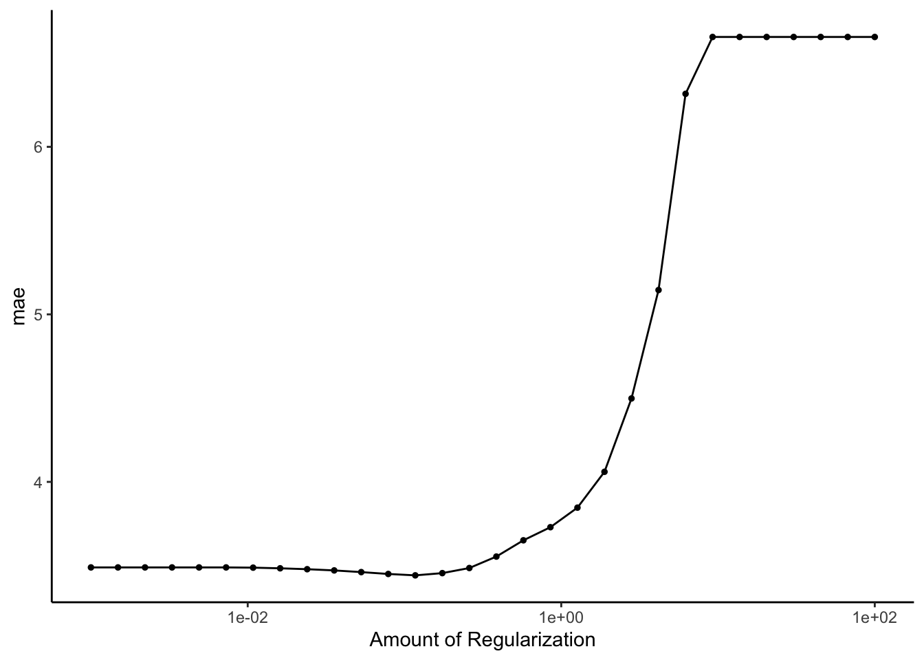
To begin our second model, we must first tune our penalty term, \(\lambda\). The visualization shows the value of the penalty term along the x-axis and the cross-validated MAE values on the y-axis.
## # A tibble: 8 × 3
##   term        estimate penalty
##   <chr>          <dbl>   <dbl>
## 1 (Intercept)  22.4      0.574
## 2 crim         -0.0601   0.574
## 3 rm            2.95     0.574
## 4 dis          -0.0344   0.574
## 5 ptratio      -1.56     0.574
## 6 b             0.487    0.574
## 7 lstat        -3.61     0.574
## 8 chas_X1       1.39     0.574
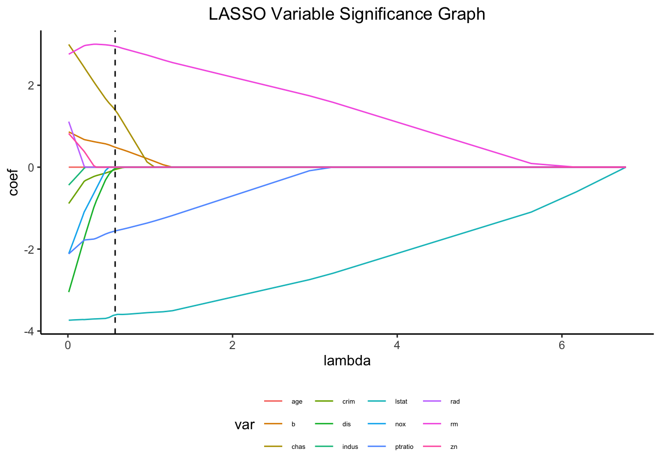
The dotted line of our LASSO variable significance graph is our penalty term, \(\lambda\) = 0.5736153. We can see that only seven predictors remain after applying our penalty term: crim, rm, dis, ptratio, b, lstat, and chas_x1. We will now examine the relationships between these predictors and the outcome, medv, to determine whether or not a natural spline is necessary, except for chas_x1 as it is binary.
##
## Method: GCV   Optimizer: magic
## Smoothing parameter selection converged after 16 iterations.
## The RMS GCV score gradient at convergence was 1.344817e-06 .
## The Hessian was positive definite.
## Model rank =  56 / 56
##
## Basis dimension (k) checking results. Low p-value (k-index<1) may
## indicate that k is too low, especially if edf is close to k'.
##
##              k'  edf k-index p-value
## s(crim)    9.00 1.47    1.03   0.780
## s(rm)      9.00 7.35    0.90   0.020 *
## s(dis)     9.00 8.66    0.99   0.330
## s(ptratio) 9.00 3.81    0.65  <2e-16 ***
## s(b)       9.00 6.28    0.94   0.085 .
## s(lstat)   9.00 5.83    1.01   0.565
## ---
## Signif. codes:  0 '***' 0.001 '**' 0.01 '*' 0.05 '.' 0.1 ' ' 1
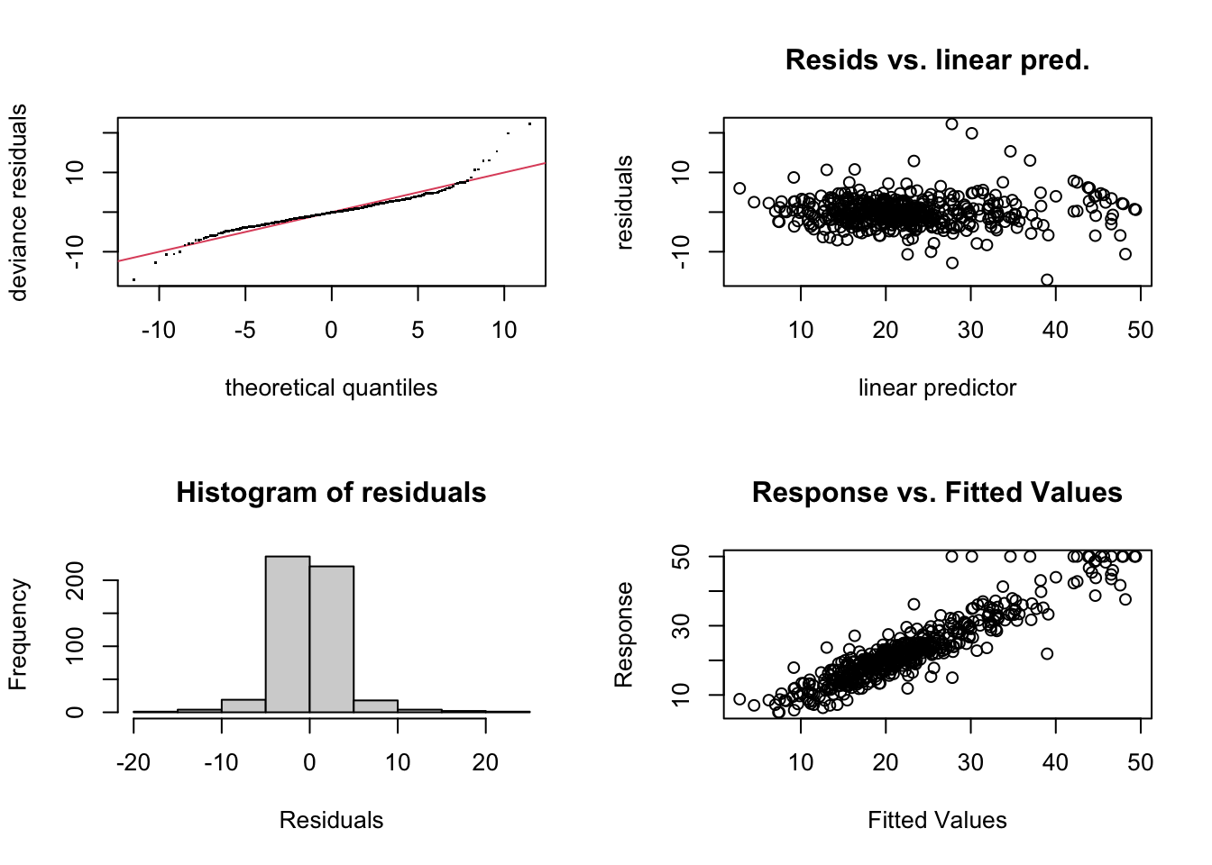
There are no extreme patterns in the Q-Q plot, and since they are close to the line, we know that the residuals are approximately normal. The residuals versus linear prediction plot looks relatively fine, and the histogram of the residuals plot is normal, which is ideal. Finally, the response versus fitted values is positively correlated, which they should be.
##
## Family: gaussian
## Link function: identity
##
## Formula:
## medv ~ chas + s(crim) + s(rm) + s(dis) + s(ptratio) + s(b) +
##     s(lstat)
##
## Parametric coefficients:
##             Estimate Std. Error t value Pr(>|t|)
## (Intercept)  22.4053     0.1717 130.489  < 2e-16 ***
## chas1         1.8433     0.6900   2.671  0.00781 **
## ---
## Signif. codes:  0 '***' 0.001 '**' 0.01 '*' 0.05 '.' 0.1 ' ' 1
##
## Approximate significance of smooth terms:
##              edf Ref.df      F  p-value
## s(crim)    1.471  1.790 22.729 1.22e-06 ***
## s(rm)      7.352  8.339 22.714  < 2e-16 ***
## s(dis)     8.657  8.963  7.398  < 2e-16 ***
## s(ptratio) 3.809  4.662  6.504 1.92e-05 ***
## s(b)       6.278  7.402  2.026   0.0516 .
## s(lstat)   5.832  7.024 41.110  < 2e-16 ***
## ---
## Signif. codes:  0 '***' 0.001 '**' 0.01 '*' 0.05 '.' 0.1 ' ' 1
##
## R-sq.(adj) =  0.837   Deviance explained = 84.8%
## GCV = 14.801  Scale est. = 13.765    n = 506
From our summary, we can see that census tracts that bound the Charles River have, on average, a $1,843 higher median home value than census tracts that do not bound the Charles River, keeping all other predictors fixed. Also, based on the smooth terms, b may not be a strong predictor after considering other variables in the model. However, the p-value is nearly less than 0.05, so we will include it for now. Looking at our graphs, the relationship between the median home value and the predictors rm, dis, and lstat appear to be nonlinear, suggesting that we will need splines for these variables. We will use rounded estimated degrees of freedom to apply these natural splines and add them to the final GAM + LASSO model.
##
## Family: gaussian
## Link function: identity
##
## Formula:
## medv ~ chas + crim + s(rm) + s(dis) + ptratio + b + s(lstat)
##
## Parametric coefficients:
##              Estimate Std. Error t value Pr(>|t|)
## (Intercept) 30.677173   1.952623  15.711  < 2e-16 ***
## chas1        1.709641   0.695387   2.459   0.0143 *
## crim        -0.154559   0.025805  -5.989 4.13e-09 ***
## ptratio     -0.496793   0.097629  -5.089 5.19e-07 ***
## b            0.004106   0.002189   1.876   0.0613 .
## ---
## Signif. codes:  0 '***' 0.001 '**' 0.01 '*' 0.05 '.' 0.1 ' ' 1
##
## Approximate significance of smooth terms:
##            edf Ref.df      F p-value
## s(rm)    6.819  7.939 27.339  <2e-16 ***
## s(dis)   8.569  8.947  6.899  <2e-16 ***
## s(lstat) 5.812  7.005 41.430  <2e-16 ***
## ---
## Signif. codes:  0 '***' 0.001 '**' 0.01 '*' 0.05 '.' 0.1 ' ' 1
##
## R-sq.(adj) =  0.831   Deviance explained = 83.9%
## GCV = 15.095  Scale est. = 14.314    n = 506
Regression: Results + Conclusions
Cross-Validated Metrics
## # A tibble: 3 × 6
##   .metric .estimator  mean     n std_err .config
##   <chr>   <chr>      <dbl> <int>   <dbl> <chr>
## 1 mae     standard   3.50     10  0.235  Preprocessor1_Model1
## 2 rmse    standard   4.90     10  0.366  Preprocessor1_Model1
## 3 rsq     standard   0.721    10  0.0234 Preprocessor1_Model1

## # A tibble: 3 × 6
##   .metric .estimator  mean     n std_err .config
##   <chr>   <chr>      <dbl> <int>   <dbl> <chr>
## 1 mae     standard   2.76     10  0.154  Preprocessor1_Model1
## 2 rmse    standard   4.05     10  0.257  Preprocessor1_Model1
## 3 rsq     standard   0.804    10  0.0244 Preprocessor1_Model1
Our GAM + LASSO model has a lower cross-validated MAE, RMSE, and a higher R-Squared value than our OLS model. This means that the magnitude of the residuals is smaller for the GAM + LASSO model, and it also accounts for 80.417% of the variation in the median value of Boston owner-occupied homes per census tract compared to the OLS model’s 72.103%.
Residual Plots
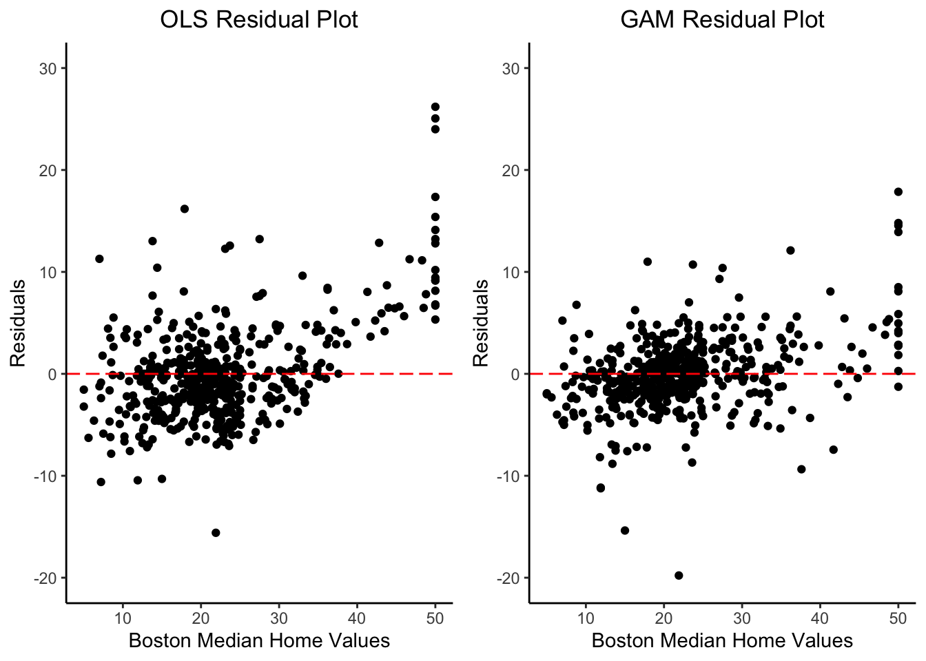
Our OLS model generally does a good job of predicting the median home values for Boston census tracts. However, we can see that our OLS model begins to underpredict median home values as they increase past 35,000 USD. From our GAM residual plot, we can see that the magnitude of the residuals is much smaller, especially for median home values that are greater than 35,000 USD.
Slope Coefficient Interpreations
## # A tibble: 27 × 5
##    term        estimate std.error statistic  p.value
##    <chr>          <dbl>     <dbl>     <dbl>    <dbl>
##  1 (Intercept) 60.4       3.68       16.4   1.98e-48
##  2 chas1        1.17      0.677       1.73  8.34e- 2
##  3 crim        -0.138     0.0251     -5.50  6.24e- 8
##  4 ptratio     -0.562     0.0942     -5.96  4.90e- 9
##  5 b            0.00364   0.00213     1.71  8.88e- 2
##  6 rm_ns_1     -1.85      2.47       -0.748 4.55e- 1
##  7 rm_ns_2     -1.02      2.67       -0.383 7.02e- 1
##  8 rm_ns_3     -1.88      2.60       -0.723 4.70e- 1
##  9 rm_ns_4     -1.86      2.61       -0.712 4.77e- 1
## 10 rm_ns_5      9.68      2.00        4.83  1.84e- 6
## # ℹ 17 more rows
crim: On average, for a 1 percent increase in per capita crime rate, the median home values of a census tract will fall by around $138, keeping all other predictors fixed.
ptratio: On average, for a 1 unit increase in the pupil-teacher ratio by census tract, the median home values will fall by around $562, keeping all other predictors fixed.
Non-linear Predictor Visualizations
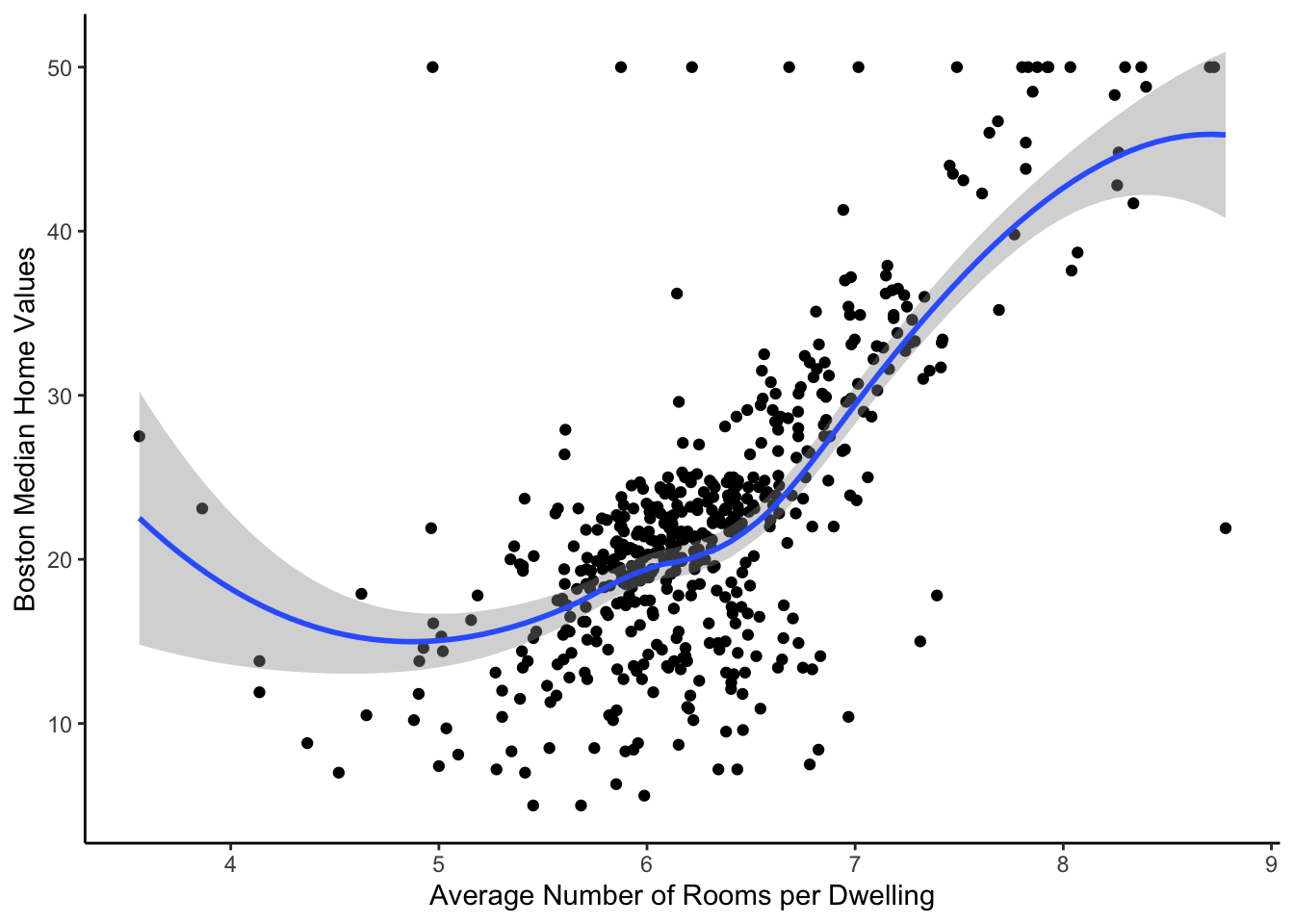
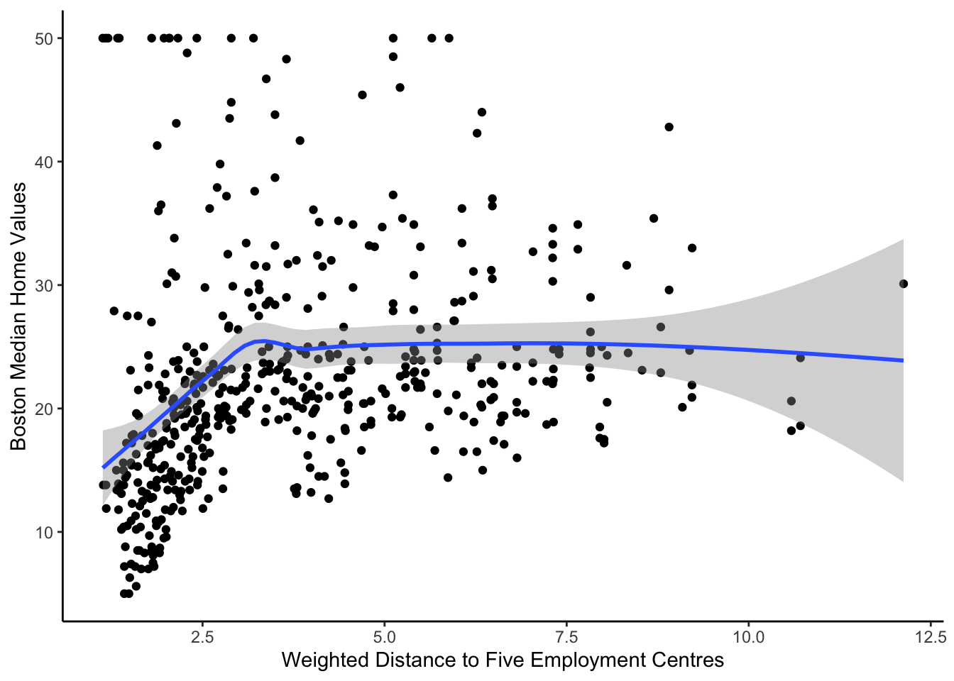
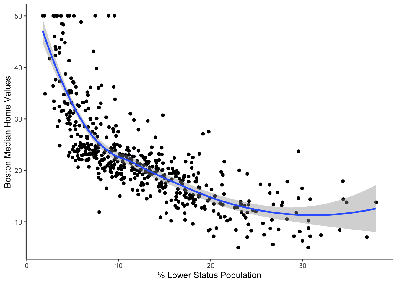
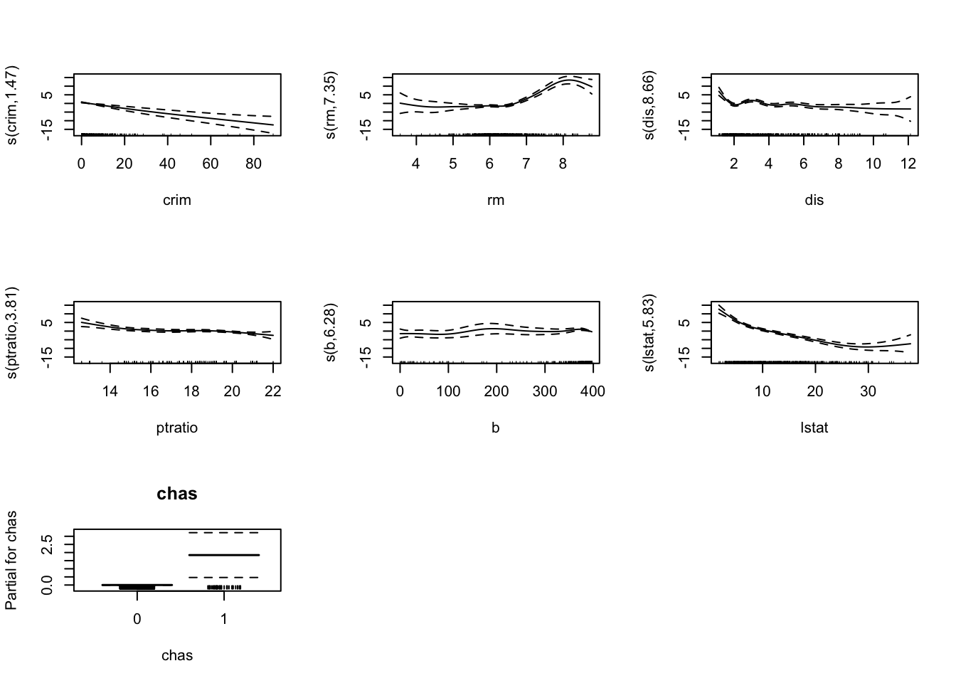
While we cannot interpret our coefficients with natural splines, we can examine their relationships with the outcome, median home values. For our first graph, rm vs. medv, we see a positive slope for dwellings with an average of 4 - 6.5 rooms. Once the average number of rooms per dwelling exceeds 6.5, the median home values increase at a faster rate. Our second graph, dis vs. medv, shows that census tracts that are closer to the five selected employment centers tend to have lower median home values until they reach a distance of 3 units. After this point, the weighted distance to the employment centers has almost no effect. Our final graph, lstat vs. medv, shows a significant negative relationship between the percentage of the lower status population and median home values that eventually flattens out as the percentage of the lower status population increases.
Conclusion
Our GAM + LASSO model does a great job examining which predictors most affect the median value of owner-occupied homes in Boston. We found that as the crime in a census tract increases, the pupil-teacher ratio increases, and the proportion of the lower status population living in a census tract increases, the median value of homes will decrease. These results indicate that we should look into the history of redlining in Boston and see if there is a correlation between neighborhoods that have been redlined in the past and a low median house value.
Classification: Methods
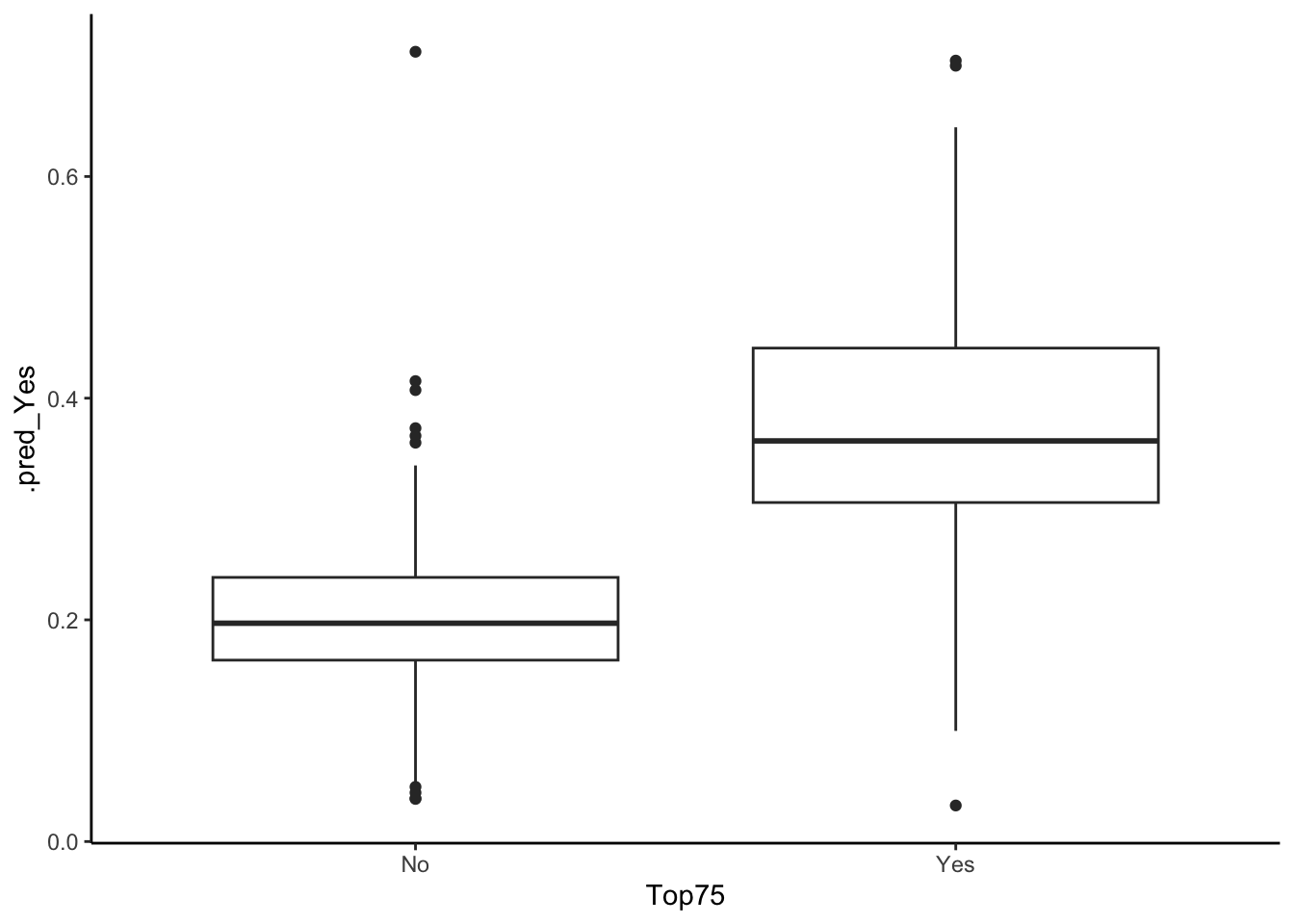
We will run a logistic LASSO and random forest to see which predictors are most useful when predicting whether or not a census tract is above or below the top 75% of Boston median home values. We created a classification data set with our new outcome variable, Top75, and we removed the medv variable as it would be taken into consideration when implementing our LASSO.
Logistic LASSO Creation
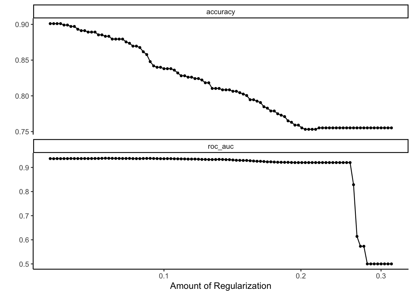
To begin our logistic LASSO model, we must first tune our penalty term, \(\lambda\). The visualization shows the value of the penalty term along the x-axis and the cross-validated accuracy and ROC_auc values on the y-axis.
## # A tibble: 3 × 3
##   term        estimate penalty
##   <chr>          <dbl>   <dbl>
## 1 (Intercept)  -1.21     0.155
## 2 rm            0.577    0.155
## 3 lstat        -0.0693   0.155

## # A tibble: 2 × 7
##   penalty .metric  .estimator  mean     n std_err .config
##     <dbl> <chr>    <chr>      <dbl> <int>   <dbl> <chr>
## 1   0.155 accuracy binary     0.795    10  0.0190 Preprocessor1_Model059
## 2   0.155 roc_auc  binary     0.928    10  0.0116 Preprocessor1_Model059
After running our LASSO using a \(\lambda\) value within one standard error of the highest cross-validated roc_auc, we have two variables remaining: rm, the average number of rooms per dwelling, and lstat, the percentage of the lower status of the population. We have a 92.789% test AUC value using these two predictors, which is promising.
##           Truth
## Prediction  No Yes
##        No  366  30
##        Yes  16  94

## # A tibble: 3 × 3
##   .metric  .estimator .estimate
##   <chr>    <chr>          <dbl>
## 1 sens     binary         0.758
## 2 spec     binary         0.958
## 3 accuracy binary         0.909
Our confusion matrix shows us that our logistic LASSO model correctly predicts 366 census tracts and incorrectly predicts 16 (false positives) of the census tracts that are not in the top 75% of Boston median home values. Furthermore, our model correctly predicts 94 census tracts and incorrectly predicts 30 census tracts (false negatives) of the census tracts in the top 75% of Boston median home values. So, of all the census tracts that are truly below the top 75% of Boston median home values, we correctly predicted 95.812% (specificity) of them. Moreover, of all the census tracts that are truly at or above the top 75% of Boston median home values, we correctly predicted 75.806% (sensitivity) of them. In the data context, we would expect to have a higher specificity than sensitivity as, inherently, there are more houses below the top 75% of Boston median home values than above, meaning that we are more likely to predict a house as below the top 75% rather than at or above this mark.
Random Forest Creation
We are going to create four random forest models. Each model will use 1000 trees and will have 2 (minimum number), 4 ($\approx \sqrt{13}$), 7 ($\approx \frac{13}{2}$), and 13 randomly sampled predictors respectively.
## # A tibble: 4 × 4
##   model  .metric  .estimator .estimate
##   <chr>  <chr>    <chr>          <dbl>
## 1 mtry2  accuracy binary         0.943
## 2 mtry4  accuracy binary         0.939
## 3 mtry7  accuracy binary         0.939
## 4 mtry13 accuracy binary         0.929
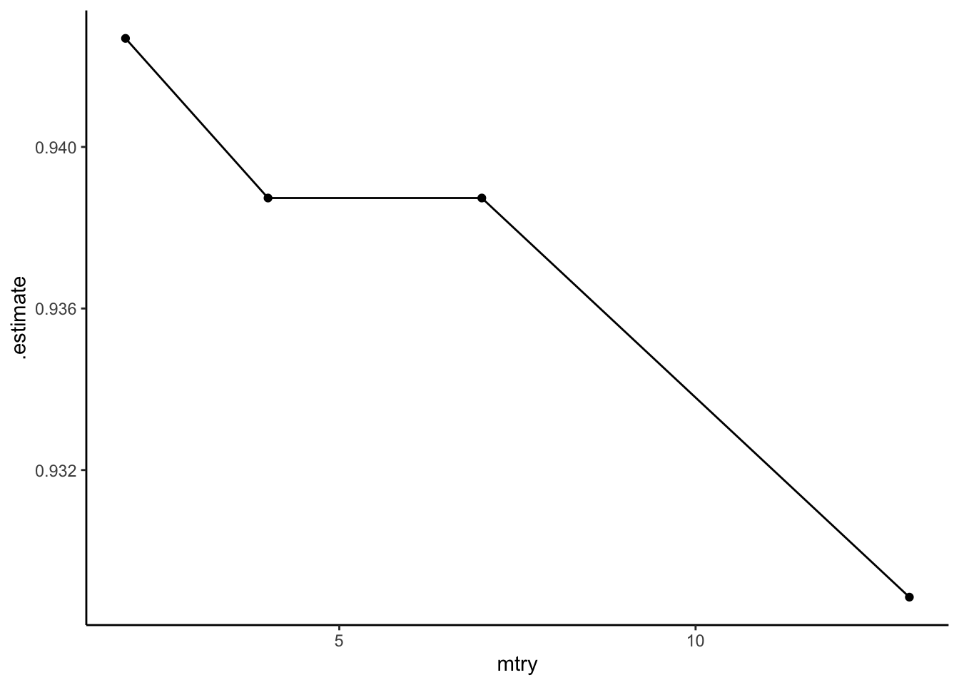
After creating creating all 4 random forest models, we have the accuracy estimates for each model. The random forest with 2 randomly sampled variables has the highest accuracy at 94.269%. The random forest models with 4 and 7 randomly sampled variables have an accuracy of 93.874%, and the model with 13 randomly sampled variables has the lowest accuracy at 92.885%.
##           Truth
## Prediction  No Yes
##        No  373  20
##        Yes   9 104

## [1] 0.8387097

## [1] 0.9764398
Our confusion matrix shows us that our random forest with two randomly sampled variables correctly predicts 373 census tracts and incorrectly predicts 9 (false positives) of the census tracts that are not in the top 75% of Boston median home values. Furthermore, our random forest correctly predicts 104 census tracts and incorrectly predicts 20 census tracts (false negatives) of the census tracts in the top 75% of Boston median home values. So, of all the census tracts that are truly below the top 75% of Boston median home values, we correctly predicted 97.644% (specificity) of them. Moreover, of all the census tracts that are truly at or above the top 75% of Boston median home values, we correctly predicted 83.871% (sensitivity) of them.
Classification: Results + Conclusions
Confusion Matrices Results
##            Model Sensitivity Specificity Overall_Accuracy
## 1 Logistic LASSO       0.758       0.958            0.909
## 2  Random Forest       0.838       0.976            0.942
When reviewing the confusion matrices for both the Logistic LASSO and random forest models, we found that our random forest model with two randomly sampled variables produces the highest sensitivity (83.8%), specificity (97.6%), and overall accuracy (94.2%). This means that our random forest model more correctly classifies census tracts above/at and below the top 75% of Boston median home values than the Logistic LASSO model.
Variable Importance
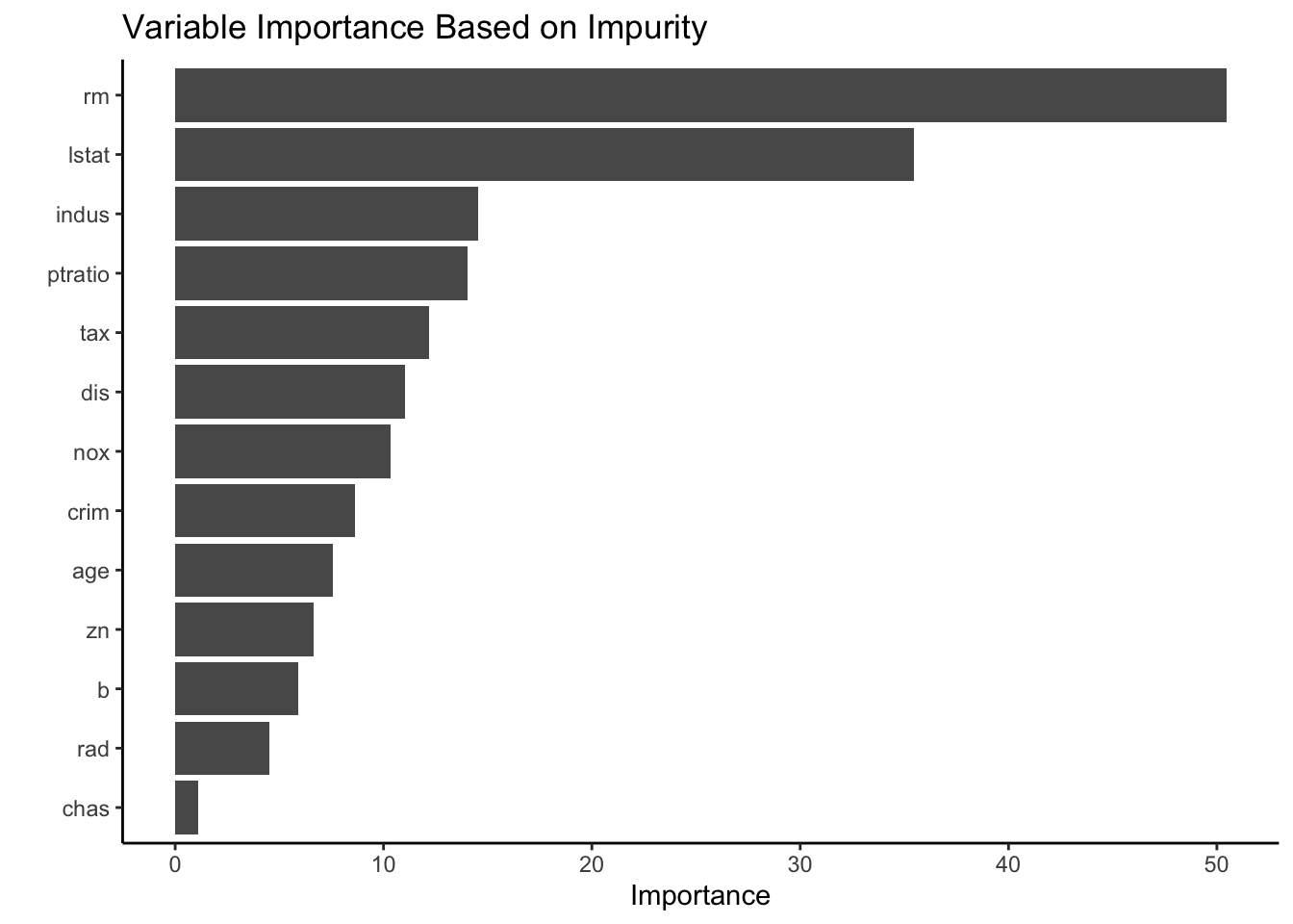
When looking at the variable importance we utilize two approaches: impurity and permutation. Our first graph shows the variable importance of the random forest model looking at the “total decrease in node impurities (as measured by the Gini index) from splitting on the variable, averaged over all trees” (Greenwell and Boehmke 2020). Using this approach, we find that rm, the average number of rooms per dwelling, and lstat, the percentage of lower status population, are considered the most important variables when classifying census tracts as either below or at/above the top 75% of Boston median home values. These predictors were also considered the most significant for our Logistic LASSO model. After two predictors, we see a large drop in importance for remaining variables.
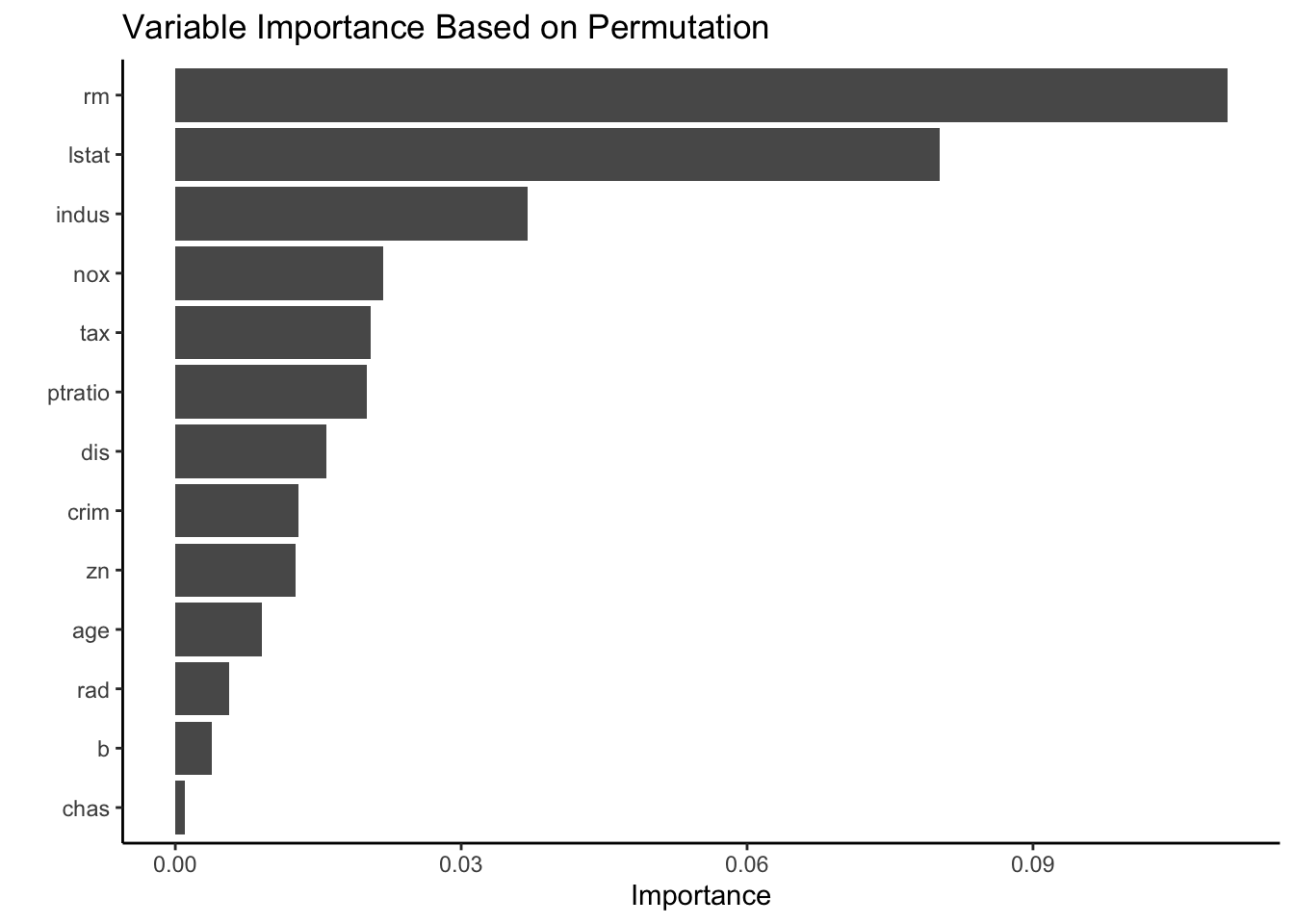
Our second graph shows a permutation approach to variable importance. We consider a variable important if it has a positive effect on the prediction performance. We find that rm and lstat are still considered to be the most important variables. Additionally, there is still a significant drop-off in variable importance between lstat and the next most important variable indus, the proportion of non-retail business acres per town. Both the impurity and permutation variable importance graphs show that chas, whether or not the census tract bounds the Charles River, has the least effect when classifying census tracts as either below or at/above the top 75% of Boston median home values.
Conclusion
Both our random forest model and our logistic LASSO model show that rm and lstat have the largest effect when determining if a census tract is below or at/above the top 75% of Boston median home values. Using our logistic LASSO Model, we found that that the estimated odds of a census tract being at/above the top 75% of Boston median home values is higher when the average number of rooms per dwelling is higher. Additionally, we found that the estimated odds of a census tract being at/above the top 75% of Boston median home values is lower when the percentage of lower status of the population of a census tract increases (which is consistent with our findings from the regression analysis). It is important to note that our random forest model found that indus was the third most important variable. While it was not included into the final model, the Boston area has struggled with industrial-caused pollution. Up until recently, Boston has had many problems with companies dropping PCBs into rivers, specifically the Neponset River in the South Boston area (Chanatry 2022). Exposure to PCBs might cause thyroid hormone toxicity in humans (“Polychlorinated Biphenyls (PCBS) Toxicity” 2014) which is why census tracts that have a smaller proportion of industrial acres might be classified as at/above 75% of Boston median home values more often.
Unsupervised Learning: Clustering
Clustering Model & Feature Selection
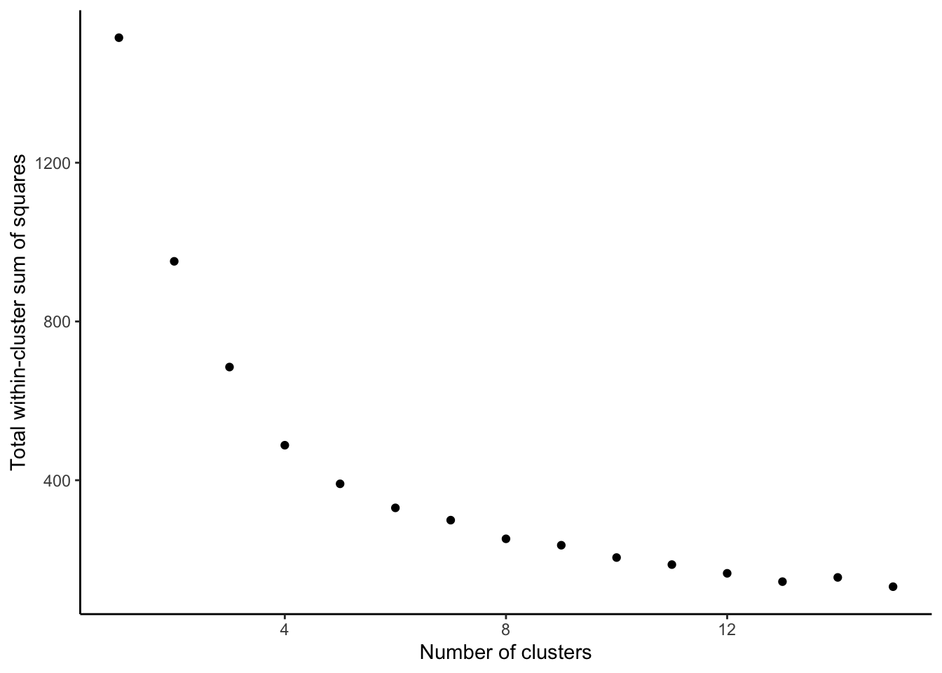
As identified earlier in the GAM + LASSO model the crime of a census tract, the pupil-teacher ratio, and the proportion of the lower status population living in a census tract have the most significant effect on the median value of homes. We would like to see if K-means clustering can identify any groups of districts which are similar and how many of those groups we may identify. In our research of finding more general clusters of districts we might want to favor parsimony - favor a fewer number of clusters.
To start, we select the variables of interest and make sure that only numeric variables are included.
K-value Choice
As we choose the k number of clusters, we want to stop at a number where we no longer see meaningful decreases in heterogeneity by increasing k. After k=4 the decreases seem to be much smaller than at lesser k values.
Visualization
We assign values of clusters to every district and create a 3-d plot, where color represents a cluster, and x,y,z coordinate represent the values of interest (crim,ptratio,lstat).
Conclusion
The plot presents an informative clustering representation of observations into 4 following groups:
-
The most notable cluster is represented by purple color, and those observations have relatively high values of x (crim), medium-high values of y (ptratio), and medium-high values of z (lstat). There are relatively few observations in this cluster, and they are best described as higher-crime districts.
-
The cluster colored in green represents observations with low values of all variables, and those can best be described by low lower-status population percentage, low crime rate, and low pupil/teacher ratio.
-
The yellow colored cluster represents observations with relatively high lower-status population percentage, but relatively low pupil/teacher ratio and crime rate.
-
The blue cluster can best be described as observations with a high pupil/teacher ratio, but low crime rates. The “lstat” values are somewhat low too.
References
Bureau, US Census. 2021. “Combining Data – a General Overview.” Census.gov. https://www.census.gov/about/what/admin-data.html.
Chanatry, Hannah. 2022. “EPA Designates Lower Neponset River in Boston and Milton a Superfund Site.” WBUR News. WBUR. https://www.wbur.org/news/2022/03/14/neponset-river-boston-superfund-epa.
Greenwell, Brandon M., and Bradley C. Boehmke. 2020. “Variable Importance Plots—an Introduction to the Vip Package.” The R Journal 12 (1): 343–66. https://doi.org/10.32614/RJ-2020-013.
“Polychlorinated Biphenyls (PCBS) Toxicity.” 2014. Centers for Disease Control and Prevention. Centers for Disease Control; Prevention. https://www.atsdr.cdc.gov/csem/polychlorinated-biphenyls/adverse_health.html.
- Posted on:
- April 25, 2022
- Length:
- 18 minute read, 3732 words
- See Also: