Identifying Risks of Brain Cancer
By Alex McCreight, Ben Christensen
December 16, 2022
Introduction
Brain cancer is one of the more deadly forms of cancer. The five-year survival rate for patients with brain tumors in the US is around 36% (Miller et al. 2021), compared to 90% for breast cancer, the most common type of cancer, and 9% for pancreatic cancer, the most deadly type of cancer (Siegel, Miller, and Jemal 2020). The incidence of brain cancer is especially high in non-Hispanic white individuals, although part of this incidence rate could result from under-sampling from minority communities (Delavar et al. 2019). While it is common in both adolescents and adults, it is important to note that it is more deadly to older populations than younger ones (Fatehi et al. 2018).
Many different factors affect survival rates among brain cancer patients. Sex can play a role in survival in the presence of surgery, with women having moderately increased rates of survival than men, but there have only been limited studies with non-uniform diagnostic standards (Le Rhun and Weller 2020). Another factor that affects survival rates is an individual’s place of residence. For example, living in a rural area is associated with lower survival than living in a metropolitan area (Delavar et al. 2019). However, studies from the United Kingdom have observed no statistically significant difference in the survival rates of people living in rural areas versus those in metropolitan areas (Tseng and Tseng 2006). We hope to explore these factors further where the research is less extensive. These tend to be the social determinants of health, where instead of the biology of the individual shaping their survival, social factors such as the wealth of a county that the individual lives in shape survival.
Biological and medical factors, such as therapies, also play a large part in shaping survival. These therapies include procedures like surgical removal of tumors or lobectomies, which is the removal of part of a lobe of the brain. They are typically related to increased patient survival (Wroński et al. 1995). Because these surgeries and interventions cost money, those with more money would have better access to them, and as such, wealthier individuals would also have higher survival. Additionally, codeletion of the 19q and 1p chromosomes is associated with higher rates of survival in brain cancer survival, especially those with glioma, a common form of brain cancer (Cairncross et al. 1998). This deletion of chromosomes can happen separately between the two, but survival is specifically related to when both are deleted (Zhao, Ma, and Zhao 2014). Codeletion is tested for through PCR testing, FISH probes, CGH, and CISH tests, all biological tests that can analyze an individual’s genome(Brandner et al. 2022). Unfortunately, the data provides no indication of which test was used, which would have been beneficial to differences in expenses and accuracy of the different types of tests. Another biological factor is where in the brain the tumor is located. The left and right hemispheres have very different functions, so in theory, there could be differences in survival between individuals with tumors in the right hemisphere versus the left hemisphere. However, the literature indicates that there is no significant difference in survival between patients with tumors in the left and right sides of the brain (Drewes et al. 2016).
This paper attempts to understand and identify survival disparities based on factors such as sex, codeletion of the 1p and 19q chromosomes, the number of tumors, the place of residence of an individual, and the age of an individual. We hope to understand the social and biological factors affecting an individual’s survival rate.
In the “Data Source” section, we discuss where we got the data and the contents of the data set. The “Code Book” provides a description of our variables. In the “Methods” section, we go over the tools we use to analyze the data and the assumptions we make when using these tools. Finally, in the “Results” section, we explore variables associated with survival and their effects through univariate Kaplan-Meier curves, multivariate log-normal and Cox PH models, and Schoenfeld residuals. In the “Discussion” section, we connect these results back to our original question and our expectations based on previous literature. In the “Conclusion” section, we recap what we found, the limitations in our analysis, and future improvements for future papers.
Data & Methods
Data Source
The data used in this project comes from the SEER*Stat Database, provided by the National Cancer Institute. Specifically, we are using the Incidence-SEER Research Data, 17 Registries, Nov 2021 Sub. The data ranges from 2000 to 2019 (Surveillance and Program 2021). It covers around 26.5% of the US population, as of the 2010 census, and around 8 million cancer patients. The 17 registries are San Francisco-Oakland SMSA, Connecticut, Hawaii, Iowa, New Mexico, Seattle (Puget Sound), Utah, Atlanta (Metropolitan), San Jose-Monterey, Los Angeles, Alaska Natives, Rural Georgia, California excluding SF/SJM/LA, Kentucky, Louisiana, New Jersey, Greater Georgia. Codeletion, a significant genetic predictor of brain cancer survival, has only been collected since 2010, and even then, testing has not been widespread, so when analyzing it, the extent of the data is even more limited.
Codebook
-
Time: Survival of patients in months.
-
Status: Whether the data is right censored or not (1 = uncensored, 0 = censored).
-
Age: Age of the patient at diagnosis (0-19, 20-39, 40-64, 65+).
-
Sex: The sex of the patient (Male or Female).
-
Surgery Result: What type of surgery the patient received if they received surgery (Local Excision, No Surgery, Excision of Mass in Brain, Partial Resection of Tumor, Unknown, Lobectomy, Full Resection of Tumor, Pathology (LITT), Excision in Spinal Cord or Nerve, Tumor Destruction (LITT)).
-
Laterality: Where in the brain the tumor is (Not a paired site, right, left, bilateral, Paired site with unknown laterality, only one side but unknown, paired site: midline tumor). Paired means that the tumor was attached to a specific nerve, lobe, or cerebrum within the brain. A non-paired site is still in the brain, but not attached to a specific part.
-
Tumor Number: The number of tumors present in the patient.
-
Codeletion: Whether or not both the 1p and 19q chromosomes have been deleted by mutation.
-
Median Household Income: The median household income of the county the patient lives in ($ 35,000, $ 35,000-54,999, $ 55,000-74,999, or greater than $ 75,000).
-
Rural-Urban Status: What type of county the patient lives in (Metropolitan Area, Non-Metropolitan, or Unknown).
Methods
Our primary analysis is done through the “survival” package in R (Therneau 2022). Using this package, we can create Kaplan-Meier curves for our data controlling for one covariate at a time. In order to plot these curves, we use the “survminer” package (Kassambara, Kosinski, and Biecek 2021). We fit a variety of log-normal and Weibull models and used likelihood ratio tests to compare the nested models and AIC to compare the non-nested models. Additionally, we fit a semi-parametric Cox PH model. To assess the validity of its PH assumption, we graphed its Schoenfeld residuals. The Kaplan-Meiers provide quick and simple visual comparisons between survival for different values of certain variables. The log-normal and Cox PH models provide numerical information on how these variables interact in the prescience of each other. Finally, the Schoenfeld residuals provide a way to assess a variable’s change in hazard over time.
The Kaplan-Meier is a non-parametric method of estimating the survival curve. For each time, \(t\), it takes the form $$\hat{S}_{t+1}=\hat{S}_{t}*\frac{N_{t+1}-D_{t+1}}{N_{t+1}}$$ where \(\hat{S}_t\) is the survival probability estimate at time \(t\), \(N_{t}\) is the number of individuals at risk at time \(t\), and \(D_{t}\) is the number of individuals who died at time \(t\)(Goel, Khanna, and Kishore 2010).
The Cox PH model is a semi-parametric method of modeling the hazard function. It is written as $$h(t)=h_0(t) e^{b_1x_1 +b_2x_2 + ... + b_k x_k}$$ where \(h_0(t)\) is the baseline hazard function, such that \(HR=\frac{h_2}{h_1}=e^{b_i},\) which allows for easy interpretation of the hazard ratio associated with the one unit change of a variable.
Results
Univariate Kaplan-Meier Plots
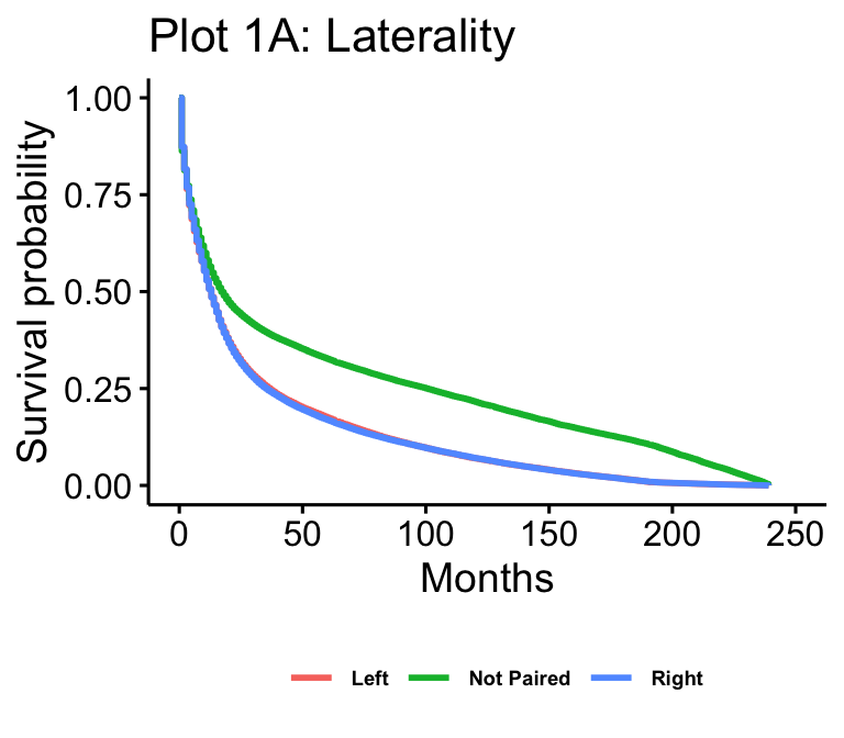
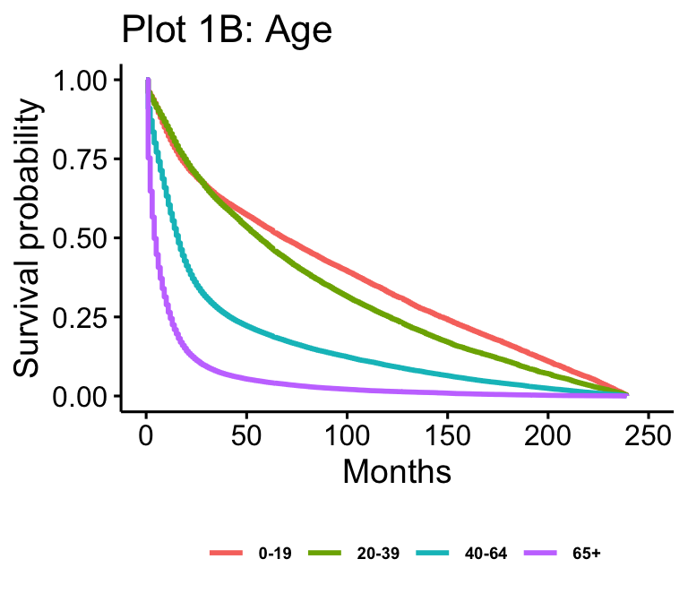
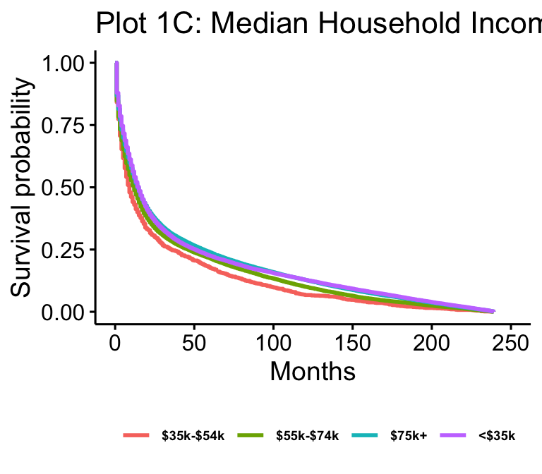
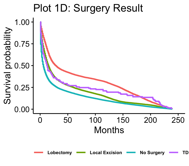
The Kaplan-Meier plots for laterality (n=102557), age (n=105538), median household income (n=105538), and surgery result (n=62822) are presented in figure 1. Age and median household income show all possible values. Laterality is reduced to just “not paired,” “right,” and “left,” which makes up over 97% of cases. Surgery result is reduced to just “Local Excision,” “No Surgery,” “Tumor Destruction (LITT),” (TD) and “Lobectomy” for readability.
Multivariate
The multivariate log-normal model of survival with age, surgery result, rural-urban status, laterality, number of tumors, sex, and median household income is presented in table 1. For concision, we only show the output for covariate values of interest, which includes all the age groups, sex, local excision, full resection, lobectomy, tumor destruction (LITT), rural-urban status, and all income groups. The youngest age group, female, no surgery, metro, and the lowest income group are the reference levels for their respective variables.
The multivariate Cox PH model of hazard with age, surgery result, rural-urban status, laterality, number of tumors, sex, and median household income is presented in table 2. Table 2 additionally has the exponentiated values for easier interpretation.
| Value | Std. Error | P-value | |
|---|---|---|---|
| Ages 20-39 | -0.114 | 0.017 | \< 0.001 |
| Ages 40-64 | -1.103 | 0.014 | \< 0.001 |
| Ages 65+ | -2.139 | 0.014 | \< 0.001 |
| SexMale | -0.09 | 0.008 | \< 0.001 |
| Local Excision | 0.527 | 0.013 | \< 0.001 |
| Full Resection | 0.485 | 0.014 | \< 0.001 |
| Lobectomy | 1.013 | 0.014 | \< 0.001 |
| Tumor Destruction (LITT) | 0.304 | 0.116 | 0.009 |
| Not Metro | 0.068 | 0.016 | \< 0.001 |
| Household Income: \$35,000 - \$54,999 | 0.156 | 0.04 | \< 0.001 |
| Household Income: \$55,000 - \$74,999 | 0.281 | 0.04 | \< 0.001 |
| Household Income: \$75,000+ | 0.333 | 0.04 | \< 0.001 |
| Value | Exp Value | Std. Error | P-value | |
|---|---|---|---|---|
| Ages 20-39 | 0.095 | 1.101 | 0.013 | \< 0.001 |
| Ages 40-64 | 0.681 | 1.977 | 0.011 | \< 0.001 |
| Ages 65+ | 1.503 | 4.501 | 0.011 | \< 0.001 |
| SexMale | 0.083 | 1.086 | 0.006 | \< 0.001 |
| Local Excision | -0.298 | 0.743 | 0.01 | \< 0.001 |
| Full Resection | -0.144 | 0.866 | 0.01 | \< 0.001 |
| Lobectomy | -0.611 | 0.543 | 0.011 | \< 0.001 |
| Tumor Destruction (LITT) | -0.32 | 0.726 | 0.087 | \< 0.001 |
| Not Metro | -0.067 | 0.935 | 0.012 | \< 0.001 |
| Household Income: \$35,000 - \$54,999 | -0.125 | 0.882 | 0.029 | \< 0.001 |
| Household Income: \$55,000 - \$74,999 | -0.233 | 0.792 | 0.03 | \< 0.001 |
| Household Income: \$75,000+ | -0.265 | 0.767 | 0.03 | \< 0.001 |
Schoenfeld Residual Plots
The Schoenfeld residual plots in plot 2 were calculated using the same Cox PH shown in table 2. We were particularly interested in assessing the validity of the PH assumption for the age and surgery variables, so we included the age 65+ group, local excision, lobectomy, and full resection plots.
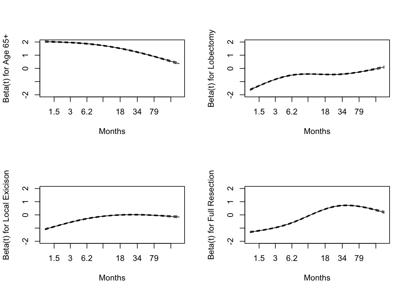
In plot 2 we see that hazard for these variables approaches zero over time.
Codeletion Kaplan-Meier
Plot 3 is the Kaplan-Meier for codeletion, performed in the same manner as plot 1.
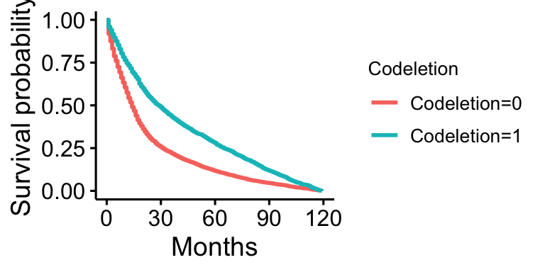 Plot 3 shows that survival is lower in those without codeletion present, and higher in those with it present.
Discusion
Kaplan-Meier Plots
Drawing from plots 1A, 1B, 1C, and 1D, we can see that many of our expectations are met without controlling for all the variables. Visually, survival is higher in younger groups (0-19 and 20-39) and lower in older groups (40-64 and 65+), which follows from intuition and past literature. The two young groups, 0-19 and 20-39, overlap early on, while survival between 40-64 and 65+ patients is further separated as we expect, with 40-64 year old patients having higher survival than 65+ year old patients. This follows our expectations.
Additionally, surgical interventions such as lobectomy, local excision, and tumor destruction (LITT) all appear to have higher survival than no surgery, at least early on. However, after about ten years, local excision drops down to around where no surgery is while tumor destruction and lobectomy still remain higher. The literature supports this result, as surgical interventions have been associated with improved survival. It is important to note, however, that surgery is very complicated, so while this appears to be the overall trend, univariate Kaplan-Meier plots do not consider confounders like age, price of surgery, or location of the tumors. All of these factors can theoretically lower survival and prevent surgery, as they can make surgery prohibitively risky and expensive. These factors are better addressed in a multivariate model where we can account for them. Interestingly, the more intrusive and sizable operations (lobectomy and tumor destruction), assuming that the patient lives through the initial procedure, appear to have much longer improvements to survival than local excision, which is a less substantial procedure.
In the case of laterality, this KM plot also generally agrees with what we expected, as left and right-paired tumors appear to have identical survival. Interestingly, non-paired tumors have much higher survival rates than their paired counterparts. There could be a few reasons for this. The first that comes to mind is that tumors paired to a side will be on areas of the brain that perform functions that are negatively impacted by the tumor and are more lethal. Another idea is that if they are not paired they could be easier to operate on or remove because you do not have to take a section of the brain out with the tumor.
The survivals between income groups appear to be much closer together than those of any other variable displayed here, with patients living in counties with median household incomes below $ 35,000 appearing to have lower survival. While the expectation might be that there would be a greater difference between income groups, this might be the case for various reasons. First, while the data gives a general picture of the resources in the county the patient lives in, it is not a complete proxy for the available resources. For example, we do not have any specific information on whether or not a patient was insured or the quality of hospitals or health care in their county. While we might assume that the quality or access to healthcare might be higher the more money a county has, this isn’t necessarily true. It might be true at the lowest levels of income, which might explain why the below $ 35,000 has lower survival, but it may not be true between counties with a medium income versus a high income.
Table 1: Log-normal Model
Our log-normal survival model supports many of the conclusions drawn from the KM plots. All the covariate values presented in Table 1 were found to be significant at the \(\alpha = 0.01\) level. We can interpret these values as a \(e^{c_k}\) for each covariate survival decreases with age as we expect, with 0-19 being the baseline, 20-39 associated with 0.89 times lower survival, 40-64 associated with 0.33 times lower survival, and 65+ being associated with 0.12 times lower survival.
The difference between income levels is more clear in the log-normal model than in the KM plot. With the poorest group as the baseline, the $ 35k - $ 55k group was associated with a 1.17 times increase in survival, the $ 55k - $ 75k with a 1.32 times increase, and $ 75+ group was associated with a 1.40 times increase. There appear to be diminishing returns on increases in income, with the difference between the two largest income groups being much smaller than the difference between the two smallest.
For surgery results, no surgery was taken as the baseline. Lobectomy had an increase of 2.75 times, local excision had an increase of 1.69 times, and total tumor destruction (LITT) had an increase of 1.36 times. Again, this supports the findings in the KM plot that the much more substantial operation in lobectomy had the highest survival increase. In contrast, smaller operations like local excision have positive but smaller increases in survival.
Sex and rural-urban status had a much smaller effect on survival, with being male being associated with a 0.91 time decrease and not living in a metro area being associated with a 1.07 times increase in survival. Fitting a model with just rural-urban status shows a decrease in survival related to not living in a metro area. However, once we control for age and income, factors that in America frequently differ across rural and urban areas, the results are flipped. The male result, while small, confirms our expectations, as we tend to expect men to live shorter on average than women, regardless of brain cancer status. However, the rural-urban difference is surprising, as one would expect that those living in urban areas live closer to hospitals and might see an improvement in this regard, but controlling for surgery results might make sense for them to be similar. Even though it is significant, the very small difference is in line with the literature, which states that there isn’t a significant difference in survival between rural and urban areas.
Table 2: Cox’s Proportional Hazard Model
Compared to individuals who were aged 0-19 years old when initially diagnosed with brain cancer, we expect to see the hazard ratio of individuals who were 65+ when diagnosed with brain cancer to have a 4.5 multiplicative increase in their hazard ratio holding all other variables constant. This agrees with previous findings, as brain cancer has a much higher mortality rate in older people than younger people (Fatehi et al. 2018).
We expect to see a 0.543 multiplicative decrease in the hazard ratio for individuals who had a lobectomy compared to individuals who did not have any surgery while holding all other variables constant. Additionally, we expect to see a 0.743 multiplicative decrease in the hazard ratio for individuals who had a local excision compared to individuals who did not have any surgery. These results align with our intuition as successful surgeries will increase brain cancer patients’ life expectancy.
Finally, we expect a 1.0861 multiplicative in the hazard ratio for males with brain cancer compared to females with brain cancer while holding all other variables constant, consistent with previous findings(Le Rhun and Weller 2020). We also found that individuals with a household income above 75,000 USD had a 0.7673 multiplicative decrease in their hazard ratio compared to individuals with a household income below 35,000 USD. Intuitively, we expected this result as people with more disposable income are more likely to have better health insurance and will be able to get higher-quality treatment and surgeries.
Schonfeld Residual Plots
We found that the highest risk of death of those originally diagnosed with brain cancer at 65 years old and older was the first few months. As time passes, the risk of death decreases, aligning with our intuition. If an individual survives the first few months, where brain cancer typically has a high mortality rate, they are more likely to be a long survivor; thus, the risk of death will decrease over time.
For individuals who had a lobectomy, local excision of their brain tumor, or a full resection of their brain tumor, their risk of death increased as time increased. This agrees with our intuition as we would expect that immediately after a successful surgery, the risk of death would be lowest and would slowly increase over time. Additionally, the severity of the procedure aligns with our intuition. For example, the rate at which the risk of death increases is faster for those who had a full resection of their brain tumor than those who had a local excision.
Final Model Selection
After reviewing the Schonfeld residual plots, we found that many of the covariates included in our model have a time-varying hazard ratio, thus violating the proportional hazard assumption of a Cox PH model. Additionally, using Akaike’s Information Criterion (AIC) we found that the log-normal model outperformed our Weibull model. So, we believe that our log-normal model more accurately captures the relationship between our covariates and the risk of death among individuals with brain cancer.
Codeletion
Our preliminary model selection for predicting survival found that codeletion was one of the best predictors of survival. The Kaplan-Meier plot for codeletion supports this. However, while it was found to be very significant and to play a large part in predicting survival, due to limitations in the data and how it was collected, it was not included in the full model. The results support preexisting literature, as those with codeletion do appear to have much higher survival than those without. Unfortunately, to keep our sample more representative of the US, we must exclude it as a predictor.
Conclusion
Summary
Our results from the Kaplan-Meier plots, a log-normal survival model, a Cox PH model, and Schonfeld residual plots all generally agree. Biological and medical factors, such as surgery result, laterality, and age, do appear to play larger parts in predicting brain cancer survival than the social determinants of health do. That being said, while rural-urban status did not play a huge factor, the income levels of the county where the patient lives did play some part, as higher income levels were associated with positive health outcomes. The health-wealth gap remains present among brain cancer patients. Considering how significant and beneficial surgery is in brain cancer and how expensive it can be, it is important to remedy this wealth gap so that patients can get the life-saving care they need.
Limitations
One limitation of our variables is that individuals are not sedentary. Their lives are not static; they move from place to place. This means that our variables, like median household income and our rural-urban continuum, fail to capture changes in their location throughout their cancer spell. Considering the sample size of data, the debilitating nature of cancer, and the fact that even if they moved, they still lived in the area represented in the data at some point, it isn’t unreasonable to assume that this locational information can still be informative, but that being said, we recognize that it is not perfect.
Another limitation of our analysis is the codeletion of the 1p and 19q chromosomes. While our literature review and analysis both support the idea that this codeletion of chromosomes is related to a significant increase in brain cancer patients’ survival, the testing has not been widely performed yet. Less than 10% of our data included testing information on it. Testing for this codeletion can be expensive, with uninsured individuals and individuals with lower incomes having the lowest reported testing rates (Zreik et al. 2021). Thus, the data set, including codeletion, does not fully represent the American population. However, because codeletion is a genetic factor, we do not expect there to be confounders, as genetics should be independent of social status. Additionally, testing only started being reported in the SEER Database in 2010 and onwards, so it has not been around for that long in the grand scheme of things. For that reason, even though we found it very significant on its own, we do not include it in our larger analysis.
Future Work
The next step in this work would be to separate the types of brain cancers and analyze each type individually instead of doing them altogether. Our work could be adapted to perform this analysis, but that much work is outside the scope of this paper. Alternatively, we could have started this paper with a smaller scope and chosen a single type of brain cancer. Also, given disparities in codeletion testing have caught up, it would be interesting to investigate further its effect on survival.
Appendex
Log-normal Univaraite Model for Rural-Urban Status
##
## Call:
## survreg(formula = Surv(Time, Status) ~ RuralUrbanBinary, data = brain2,
##     dist = "lognormal")
##                              Value Std. Error      z      p
## (Intercept)                2.63704    0.00546 482.58 <2e-16
## RuralUrbanBinaryNot Metro -0.14453    0.01611  -8.97 <2e-16
## Log(scale)                 0.50052    0.00224 223.09 <2e-16
##
## Scale= 1.65
##
## Log Normal distribution
## Loglik(model)= -447912.4   Loglik(intercept only)= -447952.6
## 	Chisq= 80.38 on 1 degrees of freedom, p= 3.1e-19
## Number of Newton-Raphson Iterations: 2
## n= 105155
References
Brandner, S., A. McAleenan, H. E. Jones, A. Kernohan, T. Robinson, L. Schmidt, S. Dawson, et al. 2022. “Diagnostic accuracy of 1p/19q codeletion tests in oligodendroglioma: A comprehensive meta-analysis based on a Cochrane systematic review.” Neuropathol Appl Neurobiol 48 (4): e12790.
Cairncross, J. G., K. Ueki, M. C. Zlatescu, D. K. Lisle, D. M. Finkelstein, R. R. Hammond, J. S. Silver, et al. 1998. “Specific genetic predictors of chemotherapeutic response and survival in patients with anaplastic oligodendrogliomas.” J Natl Cancer Inst 90 (19): 1473–79.
Delavar, A., O. M. Al Jammal, K. R. Maguire, A. R. Wali, and M. H. Pham. 2019. “The impact of rural residence on adult brain cancer survival in the United States.” J Neurooncol 144 (3): 535–43.
Drewes, C., L. M. Sagberg, A. S. Jakola, and O. Solheim. 2016. “Quality of life in patients with intracranial tumors: does tumor laterality matter?” J Neurosurg 125 (6): 1400–1407.
Fatehi, M., C. Hunt, R. Ma, and B. D. Toyota. 2018. “Persistent Disparities in Survival for Patients with Glioblastoma.” World Neurosurg 120 (December): e511–16.
Goel, M. K., P. Khanna, and J. Kishore. 2010. “Understanding survival analysis: Kaplan-Meier estimate.” Int J Ayurveda Res 1 (4): 274–78.
Kassambara, Alboukadel, Marcin Kosinski, and Przemyslaw Biecek. 2021. Survminer: Drawing Survival Curves Using ’Ggplot2’. https://CRAN.R-project.org/package=survminer.
Le Rhun, E., and M. Weller. 2020. “Sex-specific aspects of epidemiology, molecular genetics and outcome: primary brain tumours.” ESMO Open 5 (Suppl 4): e001034.
Miller, K. D., Q. T. Ostrom, C. Kruchko, N. Patil, T. Tihan, G. Cioffi, H. E. Fuchs, et al. 2021. “Brain and other central nervous system tumor statistics, 2021.” CA Cancer J Clin 71 (5): 381–406.
Siegel, R. L., K. D. Miller, and A. Jemal. 2020. “Cancer statistics, 2020.” CA Cancer J Clin 70 (1): 7–30.
Surveillance, Epidemiology, and End Results (SEER) Program. 2021. “Incidence-SEER Research Data, 17 Registries, Nov 2021 Sub.” National Cancer Institute, DCCPS, Surveillance Research Program. www.seer.cancer.gov.
Therneau, Terry M. 2022. A Package for Survival Analysis in r. https://CRAN.R-project.org/package=survival.
Tseng, J. H., and M. Y. Tseng. 2006. “Survival analysis of children with primary malignant brain tumors in England and Wales: a population-based study.” Pediatr Neurosurg 42 (2): 67–73.
Wroński, M., E. Arbit, M. Burt, and J. H. Galicich. 1995. “Survival after surgical treatment of brain metastases from lung cancer: a follow-up study of 231 patients treated between 1976 and 1991.” J Neurosurg 83 (4): 605–16.
Zhao, J., W. Ma, and H. Zhao. 2014. “Loss of heterozygosity 1p/19q and survival in glioma: a meta-analysis.” Neuro Oncol 16 (1): 103–12.
Zreik, J., P. Kerezoudis, M. A. Alvi, Y. U. Yolcu, and S. H. Kizilbash. 2021. “Disparities in Reported Testing for 1p/19q Codeletion in Oligodendroglioma and Oligoastrocytoma Patients: An Analysis of the National Cancer Database.” Front Oncol 11: 746844.
- Posted on:
- December 16, 2022
- Length:
- 21 minute read, 4392 words
- See Also: