What casues Chronic Kidney Disease of Unknown Etiology?
July 20, 2022
Introduction
This summer, I worked with Dr. Brianna Heggeseth and fellow Macalester student, Connie Zhang, researching Chronic Kidney Disease of Uncertain Etiology (CKDu) in Nicaragua. This work is in collaboration with Dr. Ben Caplin from the Department of Renal Medicine, University College London, London, UK and Dr. Marvin Gonzalez-Quiroz from the Research Centre on Health, Work and Environment, National Autonomous University of Nicaragua, León (UNAN-Leon), León, Nicaragua.
Chronic Kidney Disease of Uncertain Etiology
Chronic Kidney Disease (CKD) most commonly affects people ages 65 and older, which make up 38% of cases (“Chronic Kidney Disease in the United States” 2021.) However, young adults, ages 18-30, living in agricultural communities in Nicaragua experience Chronic Kidney Disease of Uncertain Etiology (CKDu) or Mesoamerican Nephropathy (MeN) at a significantly higher rate than the global average. We can measure kidney function using the estimated glomerular filtration rate (eGFR.) Typically, a healthy person has an eGFR level greater than 90. Someone with an eGFR measurement between 61 and 89 could still be considered healthy as long as they have relatively stable eGFR measurements across multiple check-ins (occurring every 6 to 12 months.) Once one drops below 60 eGFR at two consecutive check-ins, they will be formally diagnosed with CKD.
When investigating CKDu in agricultural communities, nephrologists are most interested in the etiology of CKDu rather than its pathogenesis. More specifically, they hope to find what causes the disease rather than what makes it worse after someone already has it. Previous studies have explored CKDu in Nicaragua but have only found the exposures that exacerbate the disease, such as outdoor agricultural work, lack of shade available during work breaks (Gonzalez-Quiroz et al. 2018,) cramps, and unintentional weight loss (Caplin et al 2022.)
Data Set
Our data comes from a community-based longitudinal study from Nicaragua’s Leon and Chinandega departments. The study has three phases dividing participants into cohorts 1, 2, and 3. Initially, check-ins took place twice a year, but after the second year of the study, the frequency was reduced to annual check-ins. Cohort 1, which began in 2015, has a male-to-female ratio of 3:1, while Cohorts 2 and 3, which began in 2018 and 2021, respectively, have an equal 1:1 male-to-female ratio. At each check-in, participants had their estimated glomerular filtration rate (eGFR), a measurement of kidney function, and other biological measurements, such as heart rate, weight, and blood pressure recorded. Additionally, participants filled out a questionnaire covering their health history, occupation history and conditions, substance history, and symptoms of sun exposure.
Growth Mixture Model
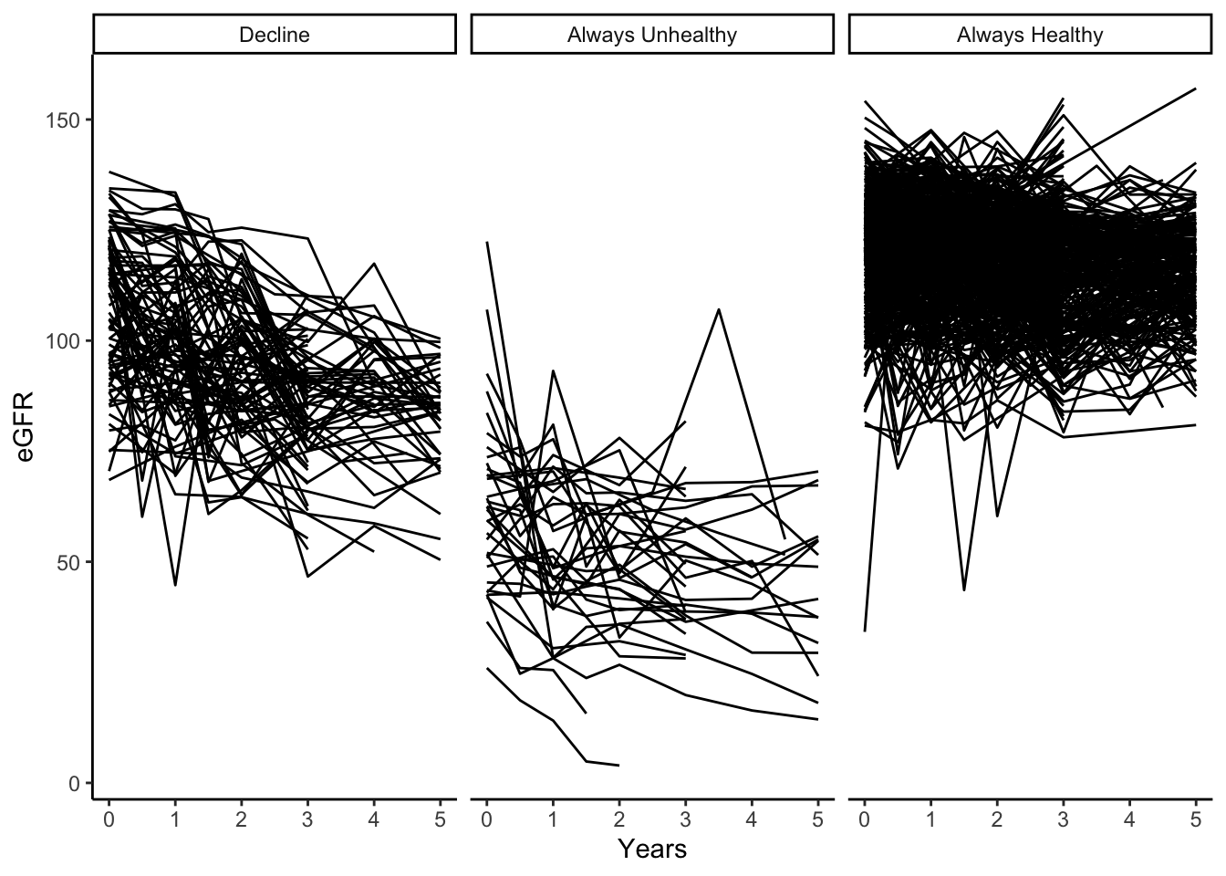
Connie primarily focused on the Growth Mixture Model (GMM) portion of our research. The GMM approach generated three latent groups of eGFR trajectories: always healthy, always unhealthy, and a rapid-decline group. The rapid-decline group was investigated for various exposures such as occupation history and conditions, substance history, and symptoms of sun exposure.
She created her best model, using a significance level of p < 0.05 and the smallest BIC score. The best model includes pregnancy, years, age, whether or not the individual worked in sugarcane since their last check-in, and whether or not an individual experienced either experienced nausea, unintentional weight loss of greater than 2.5kg, oliguria, or a headache more than once a month since their last check-in as exposures which affect an individuals mean eGFR value. Additionally, she added two variables, fever and alcohol, which affect the likelihood of being grouped into one of the three classes: always healthy, always unhealthy, or a decline in kidney function.
Hidden Markov Model
We utilized the msm package to create a continuous time hidden Markov model with two latent states, healthy and unhealthy. While we do not observe the hidden state for an individual at each check-in, we observe the initial emission distributions of the latent states. We set the initial distribution for the healthy state to have a mean eGFR level of 120 with a standard deviation of 12. For the unhealthy state, we set the mean eGFR level of 75 with a standard deviation of 15. Although stage three CKD occurs when an individual has two consecutive check-ins of a 60 eGFR or less, we set the mean just one standard deviation past this point to try to identify more people who began having a decline in kidney function to try and focus on the etiology of the disease. After defining the initial emission distributions, the HMM uses maximum likelihood estimation to create new values for the emission distributions. However, since people diagnosed with or who have had self-reported CKD were removed from the study, we had to constrain the emission distribution for the unhealthy state as there were not enough unhealthy people in our data set, causing an unhealthy mean eGFR value much higher than clinically feasible. Using these updated emission distributions, we can calculate both the joint state transition probabilities (moving from healthy to healthy, healthy to unhealthy, unhealthy to unhealthy, and unhealthy to healthy) and the posterior probabilities for each individual being in either the healthy or unhealthy state at any check-in.
We used the aforementioned initial emission distributions for our best model while constraining the unhealthy state emission distribution. We then included whether or not an individual has drunk alcohol since their previous visit, whether or not an individual has had a fever since their previous visit, an indicator variable determining if the percent change in eGFR from baseline was above or at/below 10%, and the sex of the individual. We included the sex of an individual in our analysis as many of the exposures are much more, or much less, likely depending on sex. For example, sugarcane workers and people who use alcohol are more likely to be men in our data set. All of the covariates mentioned will affect the transition probabilities, that is, the probability of transitioning from a healthy to unhealthy state or from an unhealthy to a healthy state. Finally, we took into account whether or not an individual was pregnant, as pregnancy causes an increase in eGFR levels. We determined that this model was the best as it had the lowest -2 * log likelihood value and all of the covariates included had significant hazard ratios.
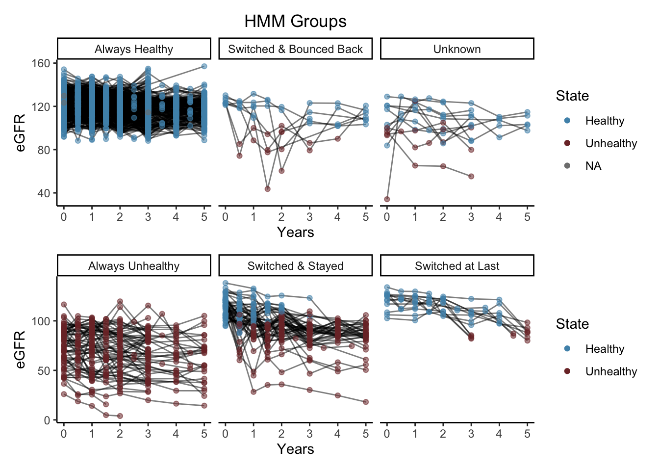
For our best HMM, we classified each individual into one of the following six groups: always healthy, always unhealthy, switched & stayed, switch & bounced back, switched at last, and unknown.
| HMM Group | Patients with… |
|---|---|
| Always Healthy | all healthy states during the study |
| Always Unhealthy | all unhealthy states during the study |
| Switched & Stayed | healthy states at the start of the study and switched to unhealthy states |
| Switched and Bounced Back | healthy states at the start of the study, switched to unhealthy state for one observation, then switched back to healthy |
| Switched at Last | healthy states throughout the study except for the last observation as unhealthy |
| Unknown | did not fit into any of the previous groups (few individuals were apart of the unknown group) |
HMM vs GMM
Our best HMM and our best GMM model included both fever and alcohol. So, for our HMM model, if an individual has had a fever or used alcohol since their last check-in, they have a higher chance of transitioning from a healthy state to an unhealthy state. For our GMM model, if an individual has had a fever or used alcohol, they are more likely to be in the decline group than the healthy group. While the two interpretations of these models are not precisely the same, they arrive at similar conclusions.
Trajectory Plots
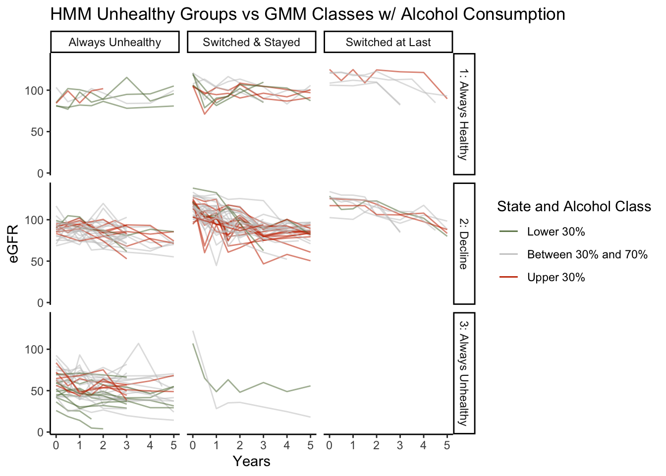
When looking at our unhealthy HMM groups, always unhealthy, switched & stayed, and switched at last, compared with the GMM classes, we found primarily complementary information. There are only four cases that our HMM deems always unhealthy and our GMM clusters into the always healthy class. Most cases that are switched & stayed are in the GMM’s eGFR decline class, which is ideal. Finally, it makes sense that the switched at last group is equally split between the always healthy class and the decline class. Depending on the severity of the drop in eGFR at an individual’s last check-in, the slope of the trajectories can be quite different, resulting in different class memberships. When looking at alcohol consumption, we see that there tend to be more individuals in the upper 30th percentile of alcohol consumption in the switched and stayed and always unhealthy HMM groups and the decline GMM group. Additionally, most individuals in the bottom 30th percentile of alcohol consumption tend to be in the always healthy GMM class.
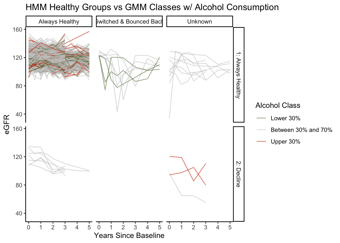
When looking at our healthy HMM groups, always healthy, switched & bounced back, and unknown, compared with the GMM classes, we found no cases where GMM records an always unhealthy class. We see that the majority of people that are always healthy and all of those who have switched and bounced back are in the always healthy class from the GMM. There are only a few cases where the HMM categorizes individuals as always healthy, and the GMM puts them into the decline class. Almost all of these cases are hovering at or below 100 eGFR, which is medically considered healthy. However, initially, they all had high eGFR readings. So, since these cases have a large negative slope, the GMM put them into the decline class. Finally, when looking at healthy individuals’ alcohol consumption, relatively few people are in the upper 30th percentile of alcohol consumption, which intuitively makes sense.
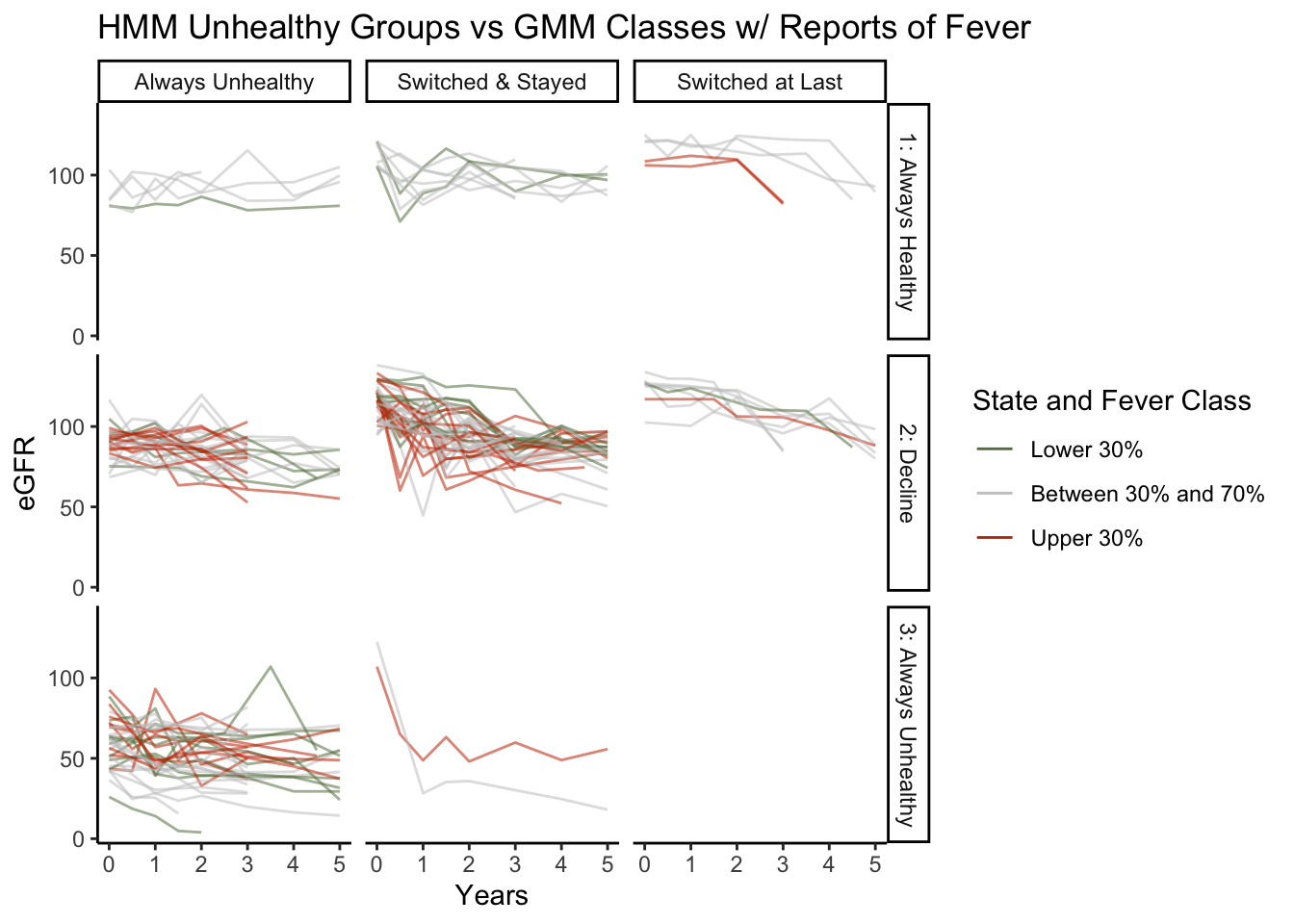
Similar to the unhealthy HMM groups and GMM class plot above, this plot considers the proportion of visits that an individual reported having a fever instead of their alcohol consumption. We see can that the GMM puts almost all individuals in the top 30th percentile of fevers reported in the decline or the always unhealthy class.
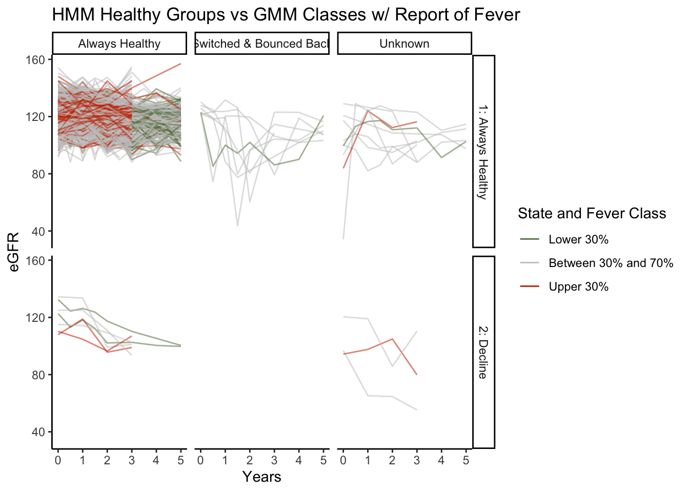
We see relatively few instances of people in the top 30th percentile of fevers reported for the healthy HMM groups. Additionally, of the seven individuals whom the GMM places into the decline in eGFR class, two are in the top 30th percentile of fevers reported.
Bar Plots
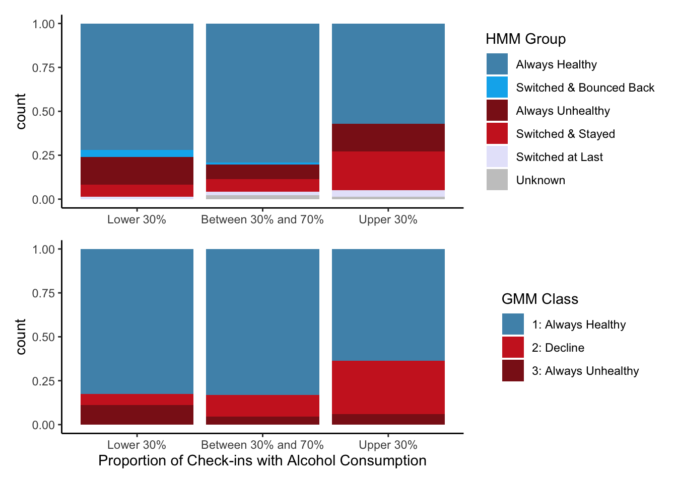
The bar plots show the proportion of each HMM group and GMM class compared with the percentile grouping of alcohol consumption. We can see very similar results from the HMM and GMM. As we move from the bottom 30th percentile toward the upper 30th percentile, the HMM is more likely to have a higher proportion of individuals in the always unhealthy or switching and staying group, and the GMM is more likely to have a higher proportion of individuals in the decline class.
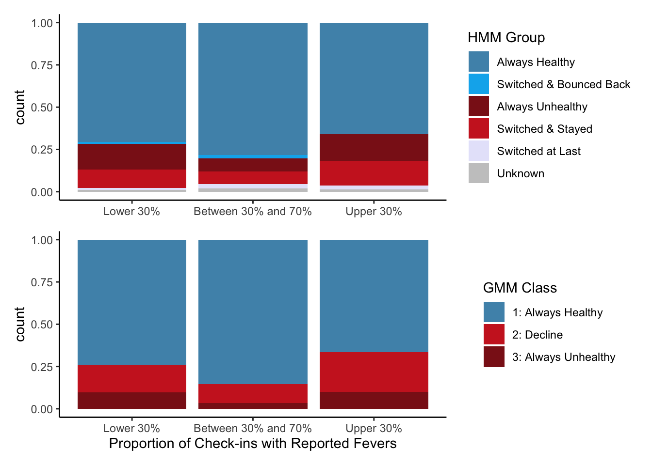
The bar plots show the proportion of each HMM group and GMM class compared with the percentile grouping of fevers reported. We can see very similar results from the HMM and GMM. As we move from the bottom 30th percentile toward the upper 30th percentile, the HMM is more likely to have a higher proportion of individuals in the always unhealthy or switching and staying group, and the GMM is more likely to have a higher proportion of individuals in the decline and always unhealthy class.
Conclusion + Future Work
Previous studies have used GMMs to evaluate the significant symptoms of CKDu. However, it was never clear whether the GMM picked up on CKDu’s etiology or its pathogenesis. Using a continuous time hidden Markov model allowed us to evaluate the probability of transitioning from a healthy to an unhealthy state. So, assuming we have correctly set up our model, increased alcohol consumption and a higher frequency of fevers lead to an increased chance of developing CKDu. Even though the GMM classifies individuals based on the slope of their eGFR trajectories, it had complementary results to the HMM’s findings. However, it is important to note that the GMM also adjusted for many other exposure variables.
In the future, we would like to add a third state to our HMM. A third state would better allow us to pick up on the time when a person initially has a decrease in kidney function but is not considered completely unhealthy. We initially tried to implement this but ran into convergence issues as we do not currently have enough data to run the model.
Acknowledgements
Thank you to Dr. Brianna Heggeseth for inviting me to this project and helping me with all my questions along the way!
Thank you to Connie Zhang ( https://connie-zhang.github.io/) for creating the GMM code, the table for the HMM group descriptions, and the HMM group visualization!
References
“Chronic Kidney Disease in the United States, 2021.” 2021. Centers for Disease Control and Prevention. Centers for Disease Control; Prevention. https://www.cdc.gov/kidneydisease/publications-resources/ckd-national-facts.html.
Gonzalez-Quiroz, Marvin, Brianna Heggeseth, Yixuan Zhang, Alexander McCreight, Armando Camacho, Amin Oomatia, Ali Al-Rashed, Nicholas Jewel, Aurora Aragon, Dorothea Nitsch, Neil Pearce, Ben Caplin. “7-year follow-up in a young adult population at risk of Mesoamerican Nephropathy: Associations with incident of chronic kidney disease and evidence of early kidney injury.”
Gonzalez-Quiroz, Marvin, Evangelia-Theano Smpokou, Richard J Silverwood, Armando Camacho, Dorien Faber, Brenda La Rosa Garcia, Amin Oomatia, et al. 2018. “Decline in Kidney Function Among Apparently Healthy Young Adults at Risk of Mesoamerican Nephropathy.” Journal of the American Society of Nephrology 29 (8): 2200–2212.
- Posted on:
- July 20, 2022
- Length:
- 11 minute read, 2185 words
- See Also: